Algorithm-Based Annotation (RCTD)

RCTD uses annotated single-cell reference data to perform cell-type deconvolution on spatial transcriptomics data, offering a practical balance between spatial resolution and cell-type resolution. In full mode, RCTD estimates the cell-type composition at each spatial location, making it particularly suitable for lower-resolution platforms such as Visium. In doublet and singlet modes, RCTD outputs dominant cell-type labels such as first_type and second_type, which are generally more interpretable in higher-resolution data.

Because RCTD results are often interpreted together with unsupervised clustering results in spatial transcriptomics studies, the pipeline outputs not only the standard deconvolution results but also comparative summaries related to the clustering structure. These include auxiliary statistics based on correlation and proportional overlap, which help assess the degree of concordance between RCTD inference and unsupervised clustering structure.

Note

1. RCTD requires raw count matrices, so both single-cell and spatial inputs should be unnormalized integer count data. If the data have been processed through the Spatialsnake pipeline, the raw expression matrix is typically preserved in the object and can be recovered.

2. It is recommended that each cell type in the single-cell reference contains at least 25 cells. Extremely rare cell types are automatically removed by the pipeline, so it is advisable to use high-quality, reliably annotated reference data.

1. Read the spatial object path and single-cell reference path from sample.txt.

2. Extract cell-type annotation information from the reference data and construct the RCTD reference object.

3. Run create.RCTD and run.RCTD on the spatial data to perform deconvolution analysis.

4. Output the main result table, weight matrix, spatial images, and other auxiliary summary files.

In short, the goal of this module is to use a high-quality single-cell reference to estimate the cell-type composition, or dominant cell type, at each spatial location and thereby support subsequent spatial interpretation and clustering comparison.

RCTD generally requires the following two types of inputs:

1. A spatial transcriptomics object in .h5ad format. Because RCTD is not suitable for direct multi-sample integrated analysis, multi-sample spatial data should typically be split by sample and run individually first.

2. A single-cell reference object in .rds format. In the example data, the public data are provided as an annotation table and HDF5 files, so they need to be assembled into an annotated .rds reference object first.

Here we use the spatial object generated in Spatialsnake for multi-sample integration as an example, together with the six accompanying single-cell files from the published study.

If you are currently using a multi-sample integrated spatial object, please first use our utility tools to split the data, then convert zarr to h5ad for use in the R-based RCTD pipeline:

step 1: sample.txt configuration file

sample.txt must contain at least the spatial object path and the single-cell reference path.

sample_id   input_path                                      sc_reference
ST8059052   results/useful_results/ST8059052.h5ad           data/merged_sc_with_annotation.rds

Step 2: Parameter Selection and Configuration

The following parameters are usually the highest priority to confirm when running RCTD:

Parameter	Example	Description
RCTD_mode	full / doublet	Specifies the RCTD prediction mode; full is better suited for lower-resolution spatial data, doublet is more appropriate when focusing on dominant cell-type combinations
sc_cell_type_col	annotation_1	Column name storing cell-type labels in the single-cell reference object
spatial_cell_type_col	celltype	Column name of existing annotation in the spatial object, used for reference display or downstream comparison
group_by	sample	Column name used for grouped summaries or comparisons, often used for sample-level organization
max_cores	8	Upper limit for parallel computing cores
threads	64	Number of backend threads; affects overall runtime
zarr_input	results/useful_results/ST8059052.zarr	If the original zarr object is available, providing it generally facilitates writing results back for spatial visualization

Configuration recommendations:

1. RCTD_mode is one of the most critical parameters. If the goal is to estimate cell-type composition at each spot, full is usually the preferred choice; if the focus is on dominant cell types and doublet inference, doublet may be considered.

2. sc_cell_type_col must match the actual annotation column name in the reference object; otherwise RCTD cannot correctly identify reference cell types.

3. If further spatial visualization of results is desired, it is recommended to retain or supplement zarr_input to facilitate writing results back to an object better suited for spatial display.

A typical configuration example:

threads: 64
RCTD_mode: "full"
sc_cell_type_col: "annotation_1"
spatial_cell_type_col: "celltype"
group_by: "sample"
max_cores: 8
zarr_input: ""

Step 3: Run the Command

Ensure that annotation.yaml and sample.txt are ready in the working directory, then run:

spatialsnake single_analysis sample.txt visium --option=annotation --anno_algorithm=RCTD --configfile=annotation.yaml --zarr_input="results/useful_results/ST8059052.h5ad"

Using the six single-cell files from the example study, the following demonstrates how to build the reference object required for RCTD and run the pipeline.

1. Prepare the spatial transcriptomics data

# If the data are already single-sample, the splitting step can be skipped
spatialsnake useful_tool --option=splitting results/merge_data/annotation/concatenated_sdata.zarr --split_by=sample

# Convert zarr to h5ad for use in the RCTD workflow
spatialsnake useful_tool --option=transform results/useful_results/ST8059052.zarr --transform_from=zarr --transform_to=h5ad --save_image=True --output_dir=results/useful_results

2. Prepare the single-cell transcriptomics data

Similarly, we use the six mouse brain single-cell data from the accompanying publication. Create and run the download script in your working directory to download the six single-cell reference files and the annotation table to data/sc_data.

Create the script file:

#!/usr/bin/env bash
set -euo pipefail

ids=(
  5705STDY8058280
  5705STDY8058281
  5705STDY8058282
  5705STDY8058283
  5705STDY8058284
  5705STDY8058285
)

mkdir -p "data/sc_data"
cd "data/sc_data"

for id in "${ids[@]}"; do
  wget -c "https://ftp.ebi.ac.uk/biostudies/fire/E-MTAB-/115/E-MTAB-11115/Files/${id}_web_summary.html"
  wget -c "https://ftp.ebi.ac.uk/biostudies/fire/E-MTAB-/115/E-MTAB-11115/Files/${id}_filtered_feature_bc_matrix.h5"
done

wget -c "https://ftp.ebi.ac.uk/biostudies/fire/E-MTAB-/115/E-MTAB-11115/Files/cell_annotation.csv"

Run the script:

chmod +x download.sh
./download.sh

3. Build the single-cell reference object merge_anno.R

Create the reference assembly script merge_anno.R to integrate the six single-cell files and write an annotated .rds object:

library(Seurat)
library(dplyr)
h5_files <- c(
  "5705STDY8058285_filtered_feature_bc_matrix.h5",
  "5705STDY8058284_filtered_feature_bc_matrix.h5",
  "5705STDY8058283_filtered_feature_bc_matrix.h5",
  "5705STDY8058282_filtered_feature_bc_matrix.h5",
  "5705STDY8058281_filtered_feature_bc_matrix.h5",
  "5705STDY8058280_filtered_feature_bc_matrix.h5"
)
obj_list <- list()
for (f in h5_files) {
  sample_id <- sub("_filtered_feature_bc_matrix\\.h5$", "", basename(f))
  counts <- Read10X_h5(f)
  colnames(counts) <- paste0(sample_id, "_", colnames(counts))
  obj <- CreateSeuratObject(counts = counts, project = sample_id)
  obj$sample <- sample_id
  obj_list[[sample_id]] <- obj
}
merged_obj <- obj_list[[1]]
if (length(obj_list) > 1) {
  for (i in 2:length(obj_list)) {
    merged_obj <- merge(merged_obj, y = obj_list[[i]])
  }
}
anno <- read.csv("cell_annotation.csv", stringsAsFactors = FALSE, check.names = FALSE)
colnames(anno) <- trimws(colnames(anno))
anno$`Cell ID` <- trimws(as.character(anno$`Cell ID`))
anno$sample <- trimws(as.character(anno$sample))
anno$annotation_1 <- trimws(as.character(anno$annotation_1))
anno <- anno[!duplicated(anno$`Cell ID`), c("Cell ID", "sample", "annotation_1")]
rownames(anno) <- anno$`Cell ID`
meta <- merged_obj@meta.data
meta$sample <- ifelse(
  rownames(meta) %in% rownames(anno),
  anno[rownames(meta), "sample"],
  meta$sample
)
meta$annotation_1 <- ifelse(
  rownames(meta) %in% rownames(anno),
  anno[rownames(meta), "annotation_1"],
  NA
)
merged_obj@meta.data <- meta
before_n <- ncol(merged_obj)
matched_cells <- rownames(merged_obj@meta.data)[!is.na(merged_obj@meta.data$annotation_1) & merged_obj@meta.data$annotation_1 != ""]
merged_obj <- subset(merged_obj, cells = matched_cells)
after_n <- ncol(merged_obj)
DefaultAssay(merged_obj) <- "RNA"
merged_obj <- JoinLayers(merged_obj, assay = "RNA")
meta <- merged_obj@meta.data
meta$annotation_1 <- as.character(meta$annotation_1)
meta$sample <- as.character(meta$sample)
merged_obj@meta.data <- meta
saveRDS(merged_obj, file = "merged_sc_with_annotation.rds")

Run the script:

Rscript merge_anno.R

4. Configure sample.txt

sample_id   input_path                                      sc_reference
ST8059052   results/useful_results/ST8059052.h5ad           data/merged_sc_with_annotation.rds

5. Run the command

The default parameters are suitable for this example. For other datasets, verify that the cell-annotation column name is correctly specified.

spatialsnake single_analysis sample.txt visium --option=annotation --anno_algorithm=RCTD

Results and Interpretation

Result file structure

results/
└── {sample}/
    └── RCTD/
        ├── {sample}_RCTD_results.csv
        ├── {sample}_RCTD_weights.csv
        ├── {sample}.zarr/
        ├── {sample}_RCTD_spatial_plot.png
        ├── {sample}_RCTD_seurat.rds
        ├── {sample}_RCTD_full_dotplot.png
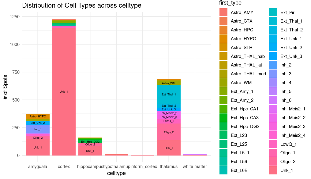
        ├── {sample}_RCTD_sample_dist_plot.png
        ├── {sample}_RCTD_cluster_plot.png
        ├── {sample}_RCTD_heatmap.png
        └── {sample}_RCTD_spot_class_bar.png

1. Primary result tables

After RCTD completes, the most important tabular outputs typically fall into the following categories:

1. {sample}_RCTD_results.csv This file is the main result table, recording the dominant predicted cell type and related allocation information for each spatial location. It serves as the basis for subsequent interpretation and statistical summary.

2. {sample}_RCTD_weights.csv This file stores the normalized weight matrix of different cell types at each spatial location. It reflects compositional structure rather than a single label, and is therefore especially suitable for mixed-location analysis, abundance comparison, and subsequent heatmap visualization.

3. {sample}_RCTD_results_all.csv or other supplementary result tables (if generated) These files typically store more detailed intermediate prediction information or auxiliary statistics, and are suitable for tracing the prediction basis for each location.

4. Summary files derived from the main results These results are typically used to generate proportion heatmaps, classification bar plots, or grouped statistical plots, reorganizing the main result table and weight matrix for easier interpretation.

In short, {sample}_RCTD_results.csv primarily answers the question “what is the most likely cell type at each location?”, while {sample}_RCTD_weights.csv is better suited for answering “which cell types constitute each location, and in what proportions?”

2. Spatial overview plot ({sample}_RCTD_spatial_plot.png)

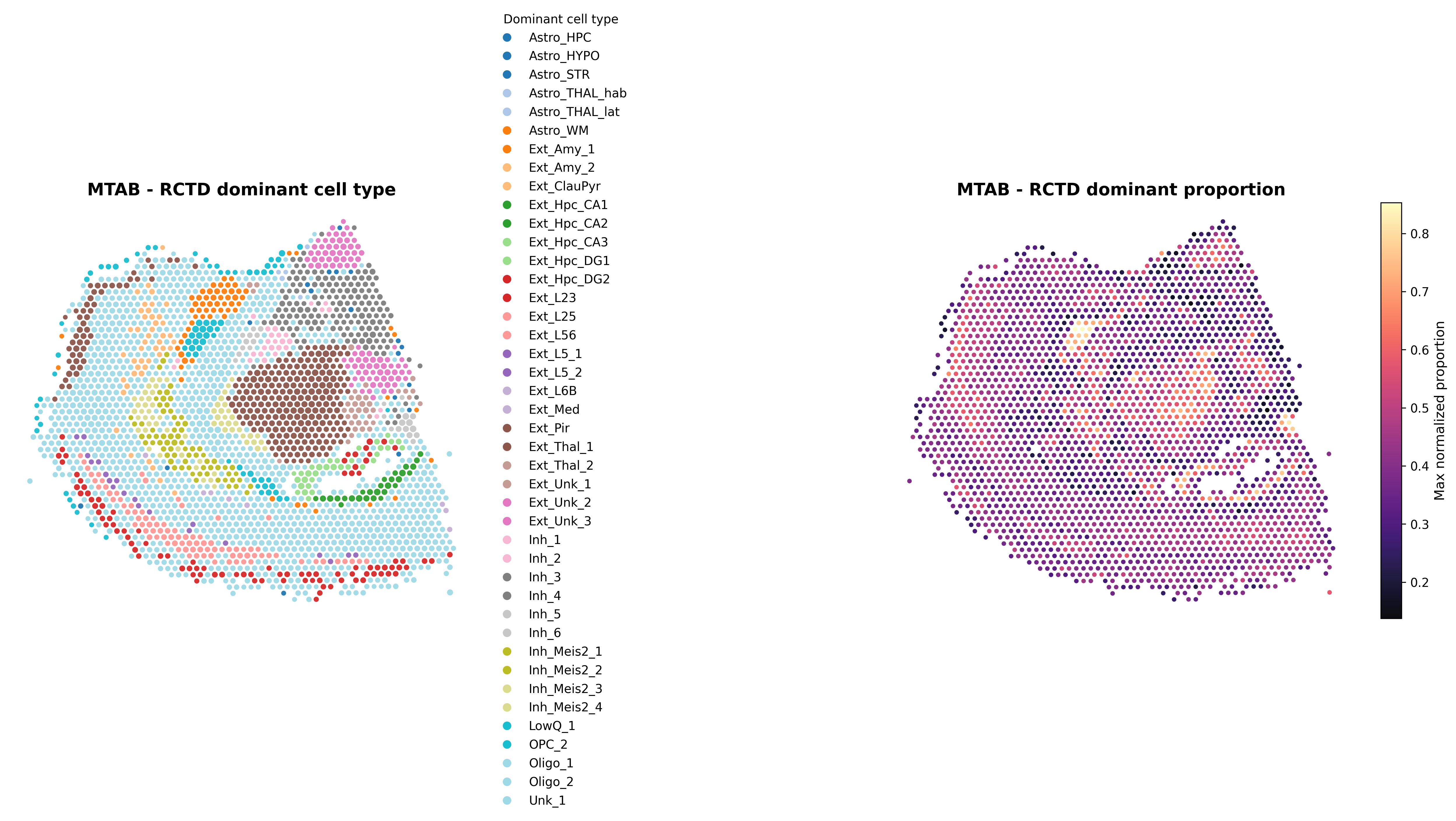
This figure provides an overall spatial view of the RCTD results, typically showing the dominant predicted cell type along with its corresponding proportion. It can be used to assess the spatial enrichment positions of different cell types in the tissue and the degree of prediction concentration.

3. Correlation dot plot ({sample}_RCTD_full_dotplot.png; key output in full mode)

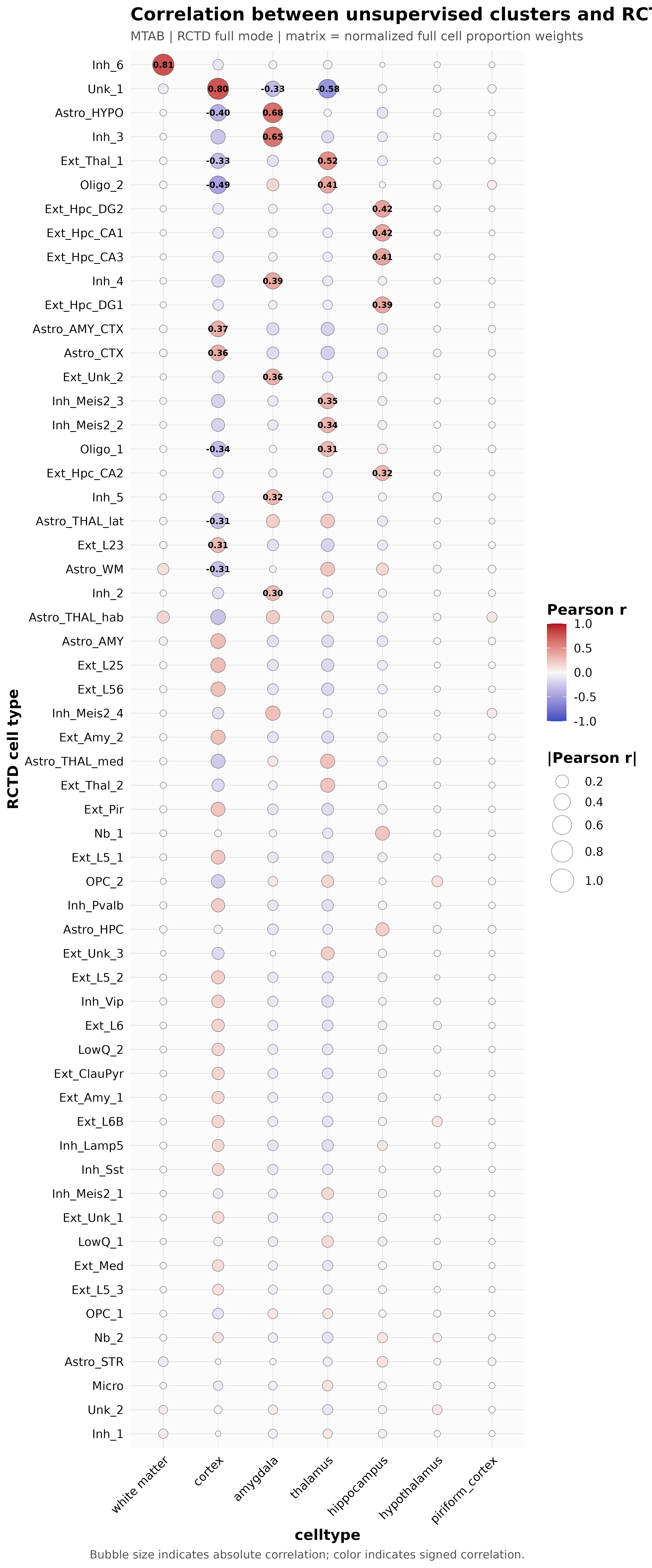
This figure is primarily used when RCTD_mode = full. The x-axis typically represents spatial clusters or user-defined groupings, and the y-axis represents reference cell types. The plot uses Pearson correlation to summarize the correspondence strength between different spatial groups and reference cell types.

4. Proportion heatmap ({sample}_RCTD_heatmap.png)

This figure is often generated in doublet mode and is especially suited for higher-resolution data. Its color intensity reflects the relative proportion of predicted cell types, and it helps compare the concordance between unsupervised clustering results and RCTD predictions.

5. Spot classification bar plot ({sample}_RCTD_spot_class_bar.png)

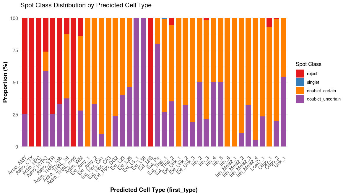
This bar plot displays the proportions of spatial locations classified as singlet, doublet, or reject, providing a concise overview of the overall classification quality for the sample.