Data Integration

This tutorial uses a Visium HD example dataset to demonstrate the full core workflow. If you are working with another spatial transcriptomics platform or with multi-sample data, go to the corresponding input tutorial and run the Ingesting step there. For the full configuration reference, see integrate.yaml Reference.

This tutorial page is intended for users who want to follow the complete core-analysis demonstration workflow. It corresponds to the same Visium HD example introduced in Visium HD Input Tutorial.

If you have already completed this step, continue directly to the preprocessing tutorial at Preprocessing.

If you are working with another platform, please return to Select your data platform and follow the corresponding ingestion tutorial there.

Demo Walkthrough

run_type: visium_HD. In this tutorial, we use the public CRC P2 dataset from the 10x Genomics website: Visium HD Human Colon Cancer P2

Visium HD data are organized by grid resolution. Each subdirectory contains the expression matrix and spatial information for one bin size, such as 2 µm, 8 µm, or 16 µm. we use the square_008um directory as the example input.

Before running Spatialsnake, create the project directory, place the downloaded Visium HD archive under data/, and extract it so that the sample folder contains binned_outputs in the expected layout. Make sure you have already created the basic working-directory structure described in the earlier setup tutorial.

Example setup:

mkdir -p project_root/data/Colon_Cancer_P2
cd project_root/data/Colon_Cancer_P2

curl -O https://cf.10xgenomics.com/samples/spatial-exp/3.0.0/Visium_HD_Human_Colon_Cancer_P2/Visium_HD_Human_Colon_Cancer_P2_binned_outputs.tar.gz
tar -xf Visium_HD_Human_Colon_Cancer_P2_binned_outputs.tar.gz

After extraction, the sample directory should match the layout shown below.

Example directory layout

project_root/
├── data/ (stores your raw data)
│   └── Colon_Cancer_P2/
├── sample.txt (key sample description file)
└── results/ (stores analysis outputs; generated automatically)

data/
└── Colon_Cancer_P2/
    └── binned_outputs/
        └── square_008um/
            ├── filtered_feature_bc_matrix.h5
            └── spatial/
                ├── tissue_positions.parquet
                ├── scalefactors_json.json
                ├── tissue_hires_image.png
                └── tissue_lowres_image.png

In this workflow, sample.txt is the key input configuration file and stores sample names together with source data paths. For this example, we use the single_analysis channel and specify the resolution in the third column. The bin value is automatically zero-padded to three digits. Make sure the sample name matches the folder name under data/:

sample_id input_path bin
Colon_Cancer_P2 data/Colon_Cancer_P2 8

Make sure sample.txt is located in your current working directory.

spatialsnake single_analysis sample.txt --option=integrate

Result file structure

results/ (under project_root)
└── Colon_Cancer_P2_008um/
    └── integrate/
        ├── Colon_Cancer_P2.zarr # zarr-formatted data
        ├── total.png # histogram of total expression
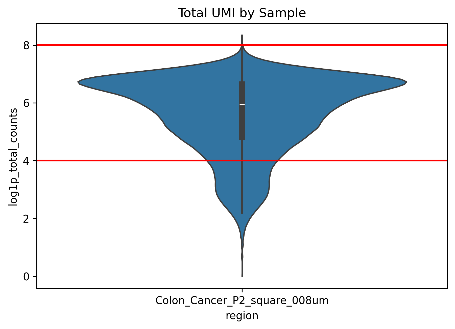
        ├── total_umi_by_sample.png # histogram of total UMI counts by sample
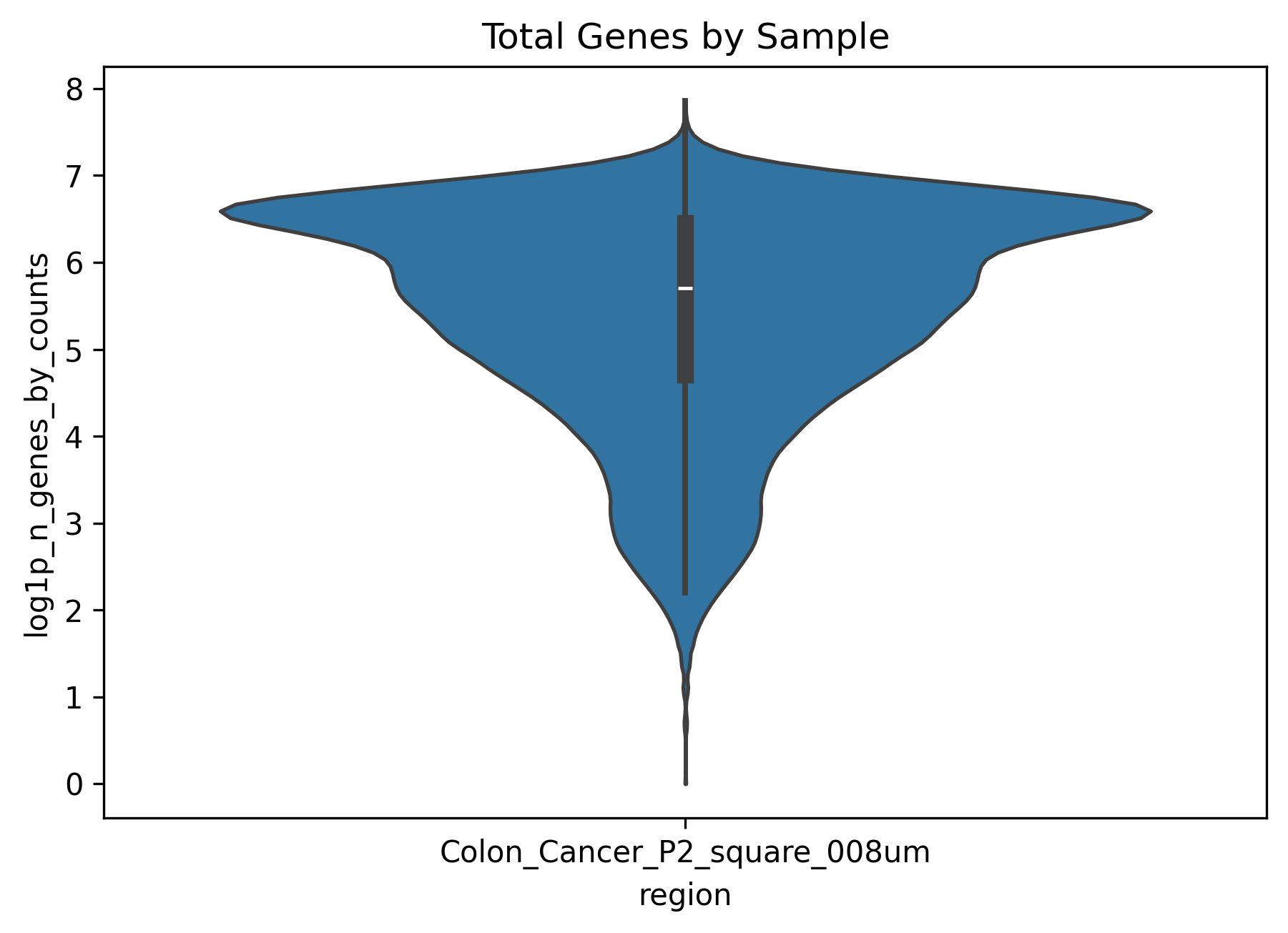
        ├── total_genes_by_sample.png # histogram of detected genes by sample
        ├── genes_by_sample.png # histogram of mitochondrial signal by sample
        └── scatter.png # scatter plot of total expression versus gene counts

How to explore the results of Ingesting?

Core outputs

• Main object: results/<sample>_<bin>um/integrate/<sample>.zarr This standardized object is used directly by subsequent steps such as preprocess and clustering. It contains the expression matrix, spatial coordinates, and sample annotation metadata.

• QC plots: total.png, total_umi_by_sample.png, total_genes_by_sample.png, genes_by_sample.png, and scatter.png in the same directory These figures are generated automatically to help you assess the overall sample state before filtering.

How to interpret the QC plots

1. total.png (overall distribution)

   • This figure is the first overall quality snapshot and helps you assess whether the sample has a clear expression signal.

   • If most observations are concentrated in the low-value range, the effective signal may be weak and the filtering thresholds in later preprocessing should be chosen carefully.

   • A small number of high-value observations can reflect locally active regions and should not automatically be treated as outliers without checking the spatial map.

2. total_umi_by_sample.png (compare total UMI across samples)

   • This figure compares whether signal intensity is in a similar range across samples.

   • If one sample is consistently much lower than the others, downstream cross-sample comparison may be strongly affected by technical differences.

   • Large differences between samples suggest that batch correction and normalization should be examined carefully in later steps.

3. total_genes_by_sample.png (compare gene complexity across samples)

   • This plot reflects how many genes are detected in each sample and can be interpreted as a measure of information richness.

   • A globally low value often suggests limited data complexity, whereas strong dispersion may indicate substantial intra-sample heterogeneity.

   • It is best interpreted together with the UMI plot rather than in isolation.

4. genes_by_sample.png (mitochondrial-related signal)

   • This plot helps identify whether the sample contains a high proportion of potentially low-quality observations.

   • If the overall level is high, more careful filtering may be required during preprocessing.

   • At the ingestion stage, the goal is to detect potential issues; actual filtering happens in the next step.

5. scatter.png (summary scatter plot)

   • This plot is useful for locating suspicious groups of observations, especially regions with low gene counts and high mitochondrial signal.

   • If most points form a continuous distribution without clear separation, the overall structure is usually relatively stable.

   • If obvious abnormal clusters appear, start with conservative filtering parameters during preprocessing and adjust gradually.

Example figures

In this example dataset, the QC plots show that some cells have very low or nearly absent expression. Based on this observation, we can apply appropriate filtering in the next step.

You have now completed the data ingestion step. Continue to Preprocessing.