Module 5: Spatially Enhanced Clustering (banksy)

banksy introduces spatial neighborhood weighting on top of expression features, thereby improving the consistency between clustering results and tissue organization. Compared with traditional clustering methods that rely solely on the expression matrix, BANKSY is better suited for identifying tissue domains with continuous spatial structure. In this tutorial, we use an already annotated example dataset to illustrate how BANKSY can reveal spatial domain structure more clearly.

For the complete parameter configuration reference, see advance_analysis.yaml Reference.

1. Read the input object and verify that spatial coordinates are complete.

2. Construct the BANKSY neighborhood graph and spatial weighting matrix.

3. Perform dimensionality reduction and spatially enhanced clustering on the weighted feature matrix.

4. If a reference annotation already exists, compare and evaluate against the non-spatial baseline clustering.

5. Output images, summary tables, and the optimal clustering labels.

More specifically, the pipeline reads a .zarr or .h5ad object and confirms the availability of spatial coordinates; if the spatial layer is missing, it attempts to reconstruct it from other coordinate fields. It then constructs a spatial neighborhood graph based on k_geom and the neighborhood decay strategy, generating weighted features that integrate neighborhood information. PCA, UMAP, and Leiden clustering are then performed under different lambda_list and resolution parameters. If a celltype label already exists in the input object, a non-spatial baseline clustering is also run, and the results are compared using metrics such as ARI, AMI, and MCC.

The recommended sample.txt format is as follows:

Input requirements:

1. The input object should contain spatial coordinate information. If missing, the pipeline will attempt to reconstruct it from fields such as array_row and array_col.

2. It is recommended to use an object that already contains celltype annotations, so that the concordance between BANKSY results and existing biological labels can be automatically compared.

step 1: sample.txt configuration file

Generally, only the sample ID and the input object path are needed to start a BANKSY analysis.

sample_id   input_path
{sample_id} results/{sample_id}/annotation/{sample_id}.zarr

Step 2: Parameter Selection and Configuration

The parameters most worth understanding first in the BANKSY module are:

Parameter	Typical values	Description
runpipe	banksy	Specifies the current advanced analysis branch as BANKSY
k_geom	15	Number of geometric neighbors; determines the local range of spatial smoothing
max_m	1	Neighborhood order; larger values place greater emphasis on more distant neighborhood information
nbr_weight_decay	scaled_gaussian	Neighborhood weight decay strategy; affects how spatial neighbors contribute to feature construction
n_comps	[20]	Number of principal components used for dimensionality reduction
lambda_list	[0.8]	Spatial weighting coefficient; larger values place greater emphasis on spatial structure information
RES	[0.5]	Leiden clustering resolution; controls clustering granularity

Configuration recommendations:

1. k_geom and lambda_list are the two most critical parameters affecting BANKSY results. The former determines the spatial neighborhood range, while the latter determines the weight of spatial information in the clustering.

2. To emphasize tissue spatial continuity more strongly, lambda_list can be moderately increased; if expression differences themselves are more important, its value can be reduced.

3. RES significantly affects the final number of spatial domains and should be chosen with consideration of tissue complexity and downstream interpretability needs.

An example configuration:

k_geom: 15
max_m: 1
nbr_weight_decay: "scaled_gaussian"
lambda_list: [0.8]

Step 3: Run the Command

Once inputs and parameters are set, run:

spatialsnake single_analysis sample.txt visium --option=advance_analysis --runpipe=banksy

Using the annotated example object, the following demonstrates the standard BANKSY analysis workflow.

1. Prepare the input object

Confirm that spatial coordinates are present in the object and, where possible, retain the celltype annotation column for subsequent comparison between spatially enhanced clustering and existing labels.

sample_id   input_path
Colon_Cancer_P2_008um results/Colon_Cancer_P2_008um/annotation/Colon_Cancer_P2.zarr

2. Set the key parameters

Focus on k_geom, lambda_list, and RES. These parameters correspond to neighborhood range, spatial weighting strength, and clustering granularity, respectively, and are critical for determining the result morphology. For this illustration, we use the default parameters.

3. Run BANKSY

spatialsnake single_analysis sample.txt visium --option=advance_analysis --runpipe=banksy

Result file structure

results/
└── banksy/
    ├── {sample}_banksy.zarr/
    ├── banksy_results/
    │   ├── banksy_results.csv
    │   ├── BANKSY-Results*.png/pdf
    │   ├── BANKSY-Results-Nonspatial*.png/pdf
    │   ├── scatter.png
    │   └── bar.png
    └── *_cell_clusters.csv

1. BANKSY spatial clustering plot

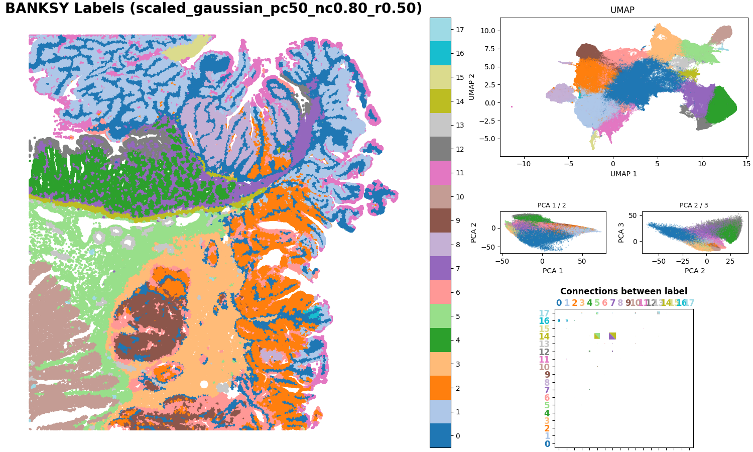
This figure displays the clustering results after incorporating spatial neighborhood weighting. Different colors correspond to different spatial domains and are primarily used to evaluate the continuity of spatial regions, boundary clarity, and consistency with tissue morphology.

2. Tissue scatter plot

This figure remaps the existing celltype annotations back onto tissue coordinates, providing a biological reference for the BANKSY clustering results.

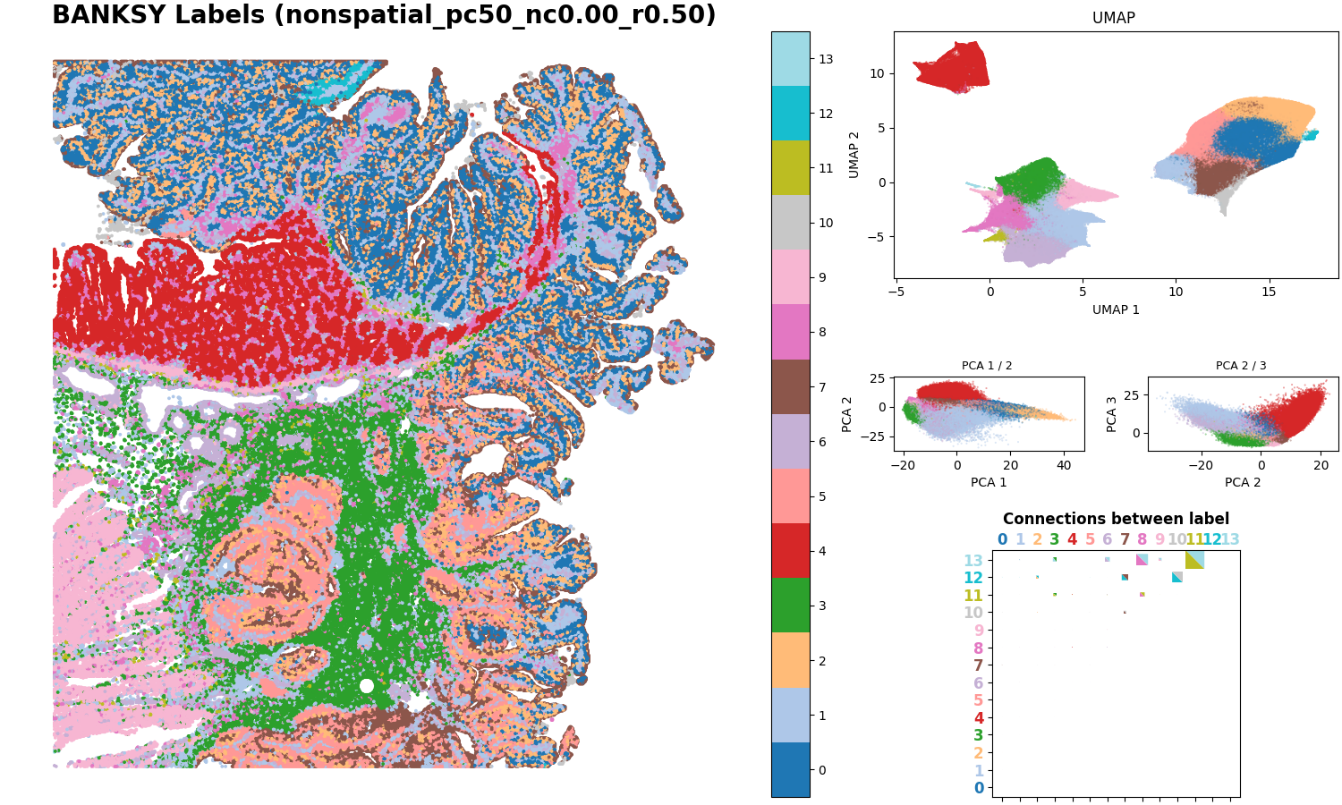
3. Non-spatial clustering comparison plot

This figure shows the clustering results when the spatial weight is set to zero, i.e., using only expression information for clustering. It helps directly compare the degree to which spatial information improves boundary smoothness and noise suppression.

4. Metric comparison bar plot

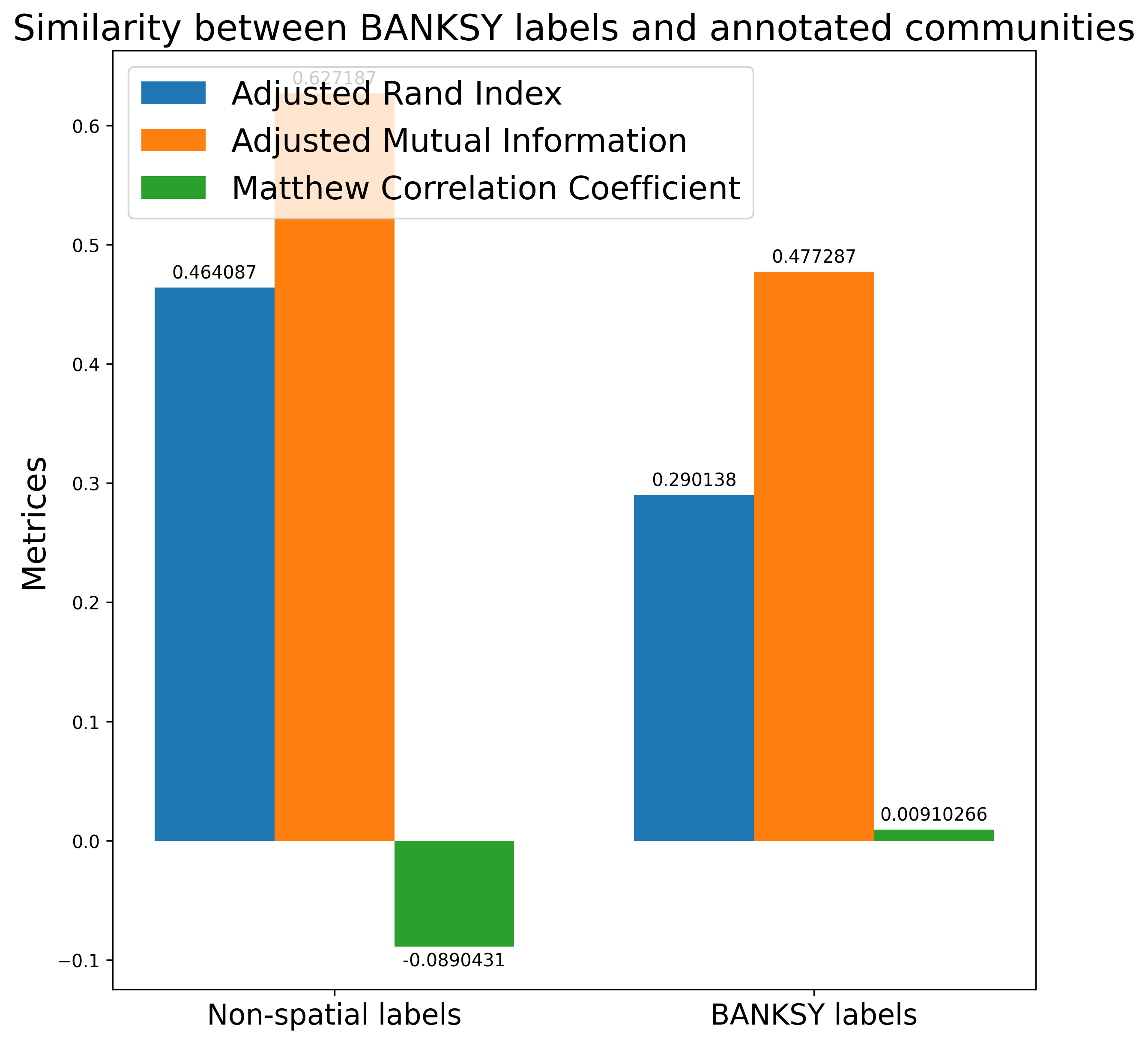
This bar plot compares spatially enhanced clustering with non-spatial clustering based on metrics such as ARI, AMI, and MCC. Higher values generally indicate better concordance between the inferred clustering results and the reference cell types or expected tissue organization.

5. Summary table of clustering labels

This table stores clustering label results for all tested parameter combinations, such as outputs corresponding to different lambda and resolution combinations. It is the core file for comparing different spatial domain granularities and ensuring result reproducibility.