Algorithm-Based Annotation (`cell2Location`)

cell2Location maps cell-type information from single-cell reference data onto spatial transcriptomic locations, thereby estimating cell-type abundance at each spatial position and generating the corresponding spatial visualizations and summary tables.

For lower-resolution spatial data such as Visium, this method is particularly well suited because it does not force a single label onto each spot, but instead estimates the proportional composition of different cell types within each spot. The method also supports annotation of spatially integrated objects from multiple samples, helping to reduce annotation inconsistency across samples. In addition to the standard cell2location outputs, the pipeline further relates the abundance results to manually defined or unsupervised clustering-derived regions, generating bubble plots and other figures to facilitate interpretation of local cell-composition patterns.

For the complete parameter configuration reference, see annotation.yaml Reference.

Read the spatial transcriptomics object (zarr) and the annotated single-cell reference object (h5ad).
Train a regression model on the reference data to learn expression signatures for different cell types.
Fit the cell2location model on the spatial object to estimate cell-type abundances at each spatial position.
Perform downstream non-negative matrix factorization (NMF) and other analyses on the abundance matrix, write results back to the object, and output visualization images, statistical summary tables, and intermediate quality-control files.

In short, the goal of this step is to use a single-cell reference to construct cell-type expression priors and map them robustly onto the spatial data, yielding cell-composition estimates for regional comparison, spatial pattern discovery, and downstream biological interpretation.

cell2Location generally requires the following two input files:

A spatial transcriptomics object in .zarr format. If you currently have only a spatial .h5ad object, please first use Format Conversion Tool (transform) to complete the format conversion.
A single-cell reference object that already contains cell-type annotation information, in .h5ad format. If you currently have only a Seurat object, please also use Format Conversion Tool (transform) to perform the conversion first.

step 1: `sample.txt` configuration file

sample.txt must contain at least the spatial object path and the single-cell reference object path.

sample_id           input_path                                      sc_reference
concatenated_sdata  results/merge_data/annotation/concatenated_sdata  data/MTAB/merged_sc_with_annotation.h5ad

Step 2: Parameter Selection and Configuration

The following table lists the commonly used parameters and their descriptions:

Parameter	Example	Description
`--anno_algorithm`	`cell2Location`	Specifies the current annotation algorithm as cell2location
`--device`	`cuda` / `cpu`	Computing device used for model training; directly affects runtime
`--image_type`	`hires`	Image layer used for spatial visualization
`--shape_type`	`cell_boundaries`	Spatial boundary layer used for overlay display
`--max_cores`	`16`	Upper limit for parallel computing resources
`max_epochs_reference`	`250`	Number of training epochs for the reference regression model
`max_epochs_st`	`30000`	Number of training epochs for the spatial model
`remove_mt`	`True`	Whether to remove mitochondrial genes before training
`N_cells_per_location`	`30`	Prior estimate of the number of cells per spatial location
`labels_key_reference`	`annotation_1`	Column name storing cell-type labels in the reference object
`batch_key_reference`	`sample`	Column name storing batch or sample information in the reference object
`batch_key_st`	`sample`	Column name storing batch or sample information in the spatial object, especially important for multi-sample integrated analyses
`cell_count_cutoff`	`15`	Cell count threshold for filtering genes in the reference data
`cell_percentage_cutoff2`	`0.05`	Cell proportion threshold for filtering genes in the reference data
`nonz_mean_cutoff`	`1.12`	Non-zero mean expression threshold for filtering genes in the reference data
`detection_alpha`	`20`	Prior parameter for the detection rate in the spatial model
`save_models`	`True`	Whether to save the reference model and spatial model directories

Configuration recommendations:

labels_key_reference, batch_key_reference, and batch_key_st are usually the parameters that should be confirmed first, as they respectively determine how cell-type labels and sample origin information are read by the model.
If the reference data comes from a multi-sample integration, it is generally recommended to set both batch_key_reference and batch_key_st to sample so that the model can correctly identify sample origins and improve cross-sample comparison reliability.
device, max_epochs_reference, and max_epochs_st significantly affect training time and can be adjusted according to hardware conditions and data scale.

If you prefer to manage parameters centrally through a configuration file, you can use annotation.yaml.

anno_algorithm: "cell2Location"
device: "cuda"
max_epochs_reference: 250
remove_mt: True
N_cells_per_location: 30
max_epochs_st: 30000
labels_key_reference: "annotation_1"
batch_key_reference: "sample"
batch_key_st: "sample"
cell_count_cutoff: 15
cell_percentage_cutoff2: 0.05
nonz_mean_cutoff: 1.12
detection_alpha: 20
save_models: True
celltype_col: "celltype"

For further YAML parameter details, see annotation.yaml Reference.

Step 3: Run the Command

Once sample.txt and the parameters are ready, run the cell2location annotation pipeline.

spatialsnake compare_analysis sample.txt visium --option=annotation --anno_algorithm=cell2Location

Using the spatial object generated in Spatialsnake for multi-sample integration as an example, together with the six accompanying single-cell files from the published study, we demonstrate how to build the reference object and perform cell2location annotation.

1. Download the reference data

Create and run a download script in your working directory to download the six single-cell reference files and their annotation table to data/sc_data. If you already have these files available, you can also manually organize them into the corresponding directory.

Create the script file:

#!/usr/bin/env bash
set -euo pipefail

ids=(
  5705STDY8058280
  5705STDY8058281
  5705STDY8058282
  5705STDY8058283
  5705STDY8058284
  5705STDY8058285
)

mkdir -p "data/sc_data"
cd "data/sc_data"

for id in "${ids[@]}"; do
  wget -c "https://ftp.ebi.ac.uk/biostudies/fire/E-MTAB-/115/E-MTAB-11115/Files/${id}_web_summary.html"
  wget -c "https://ftp.ebi.ac.uk/biostudies/fire/E-MTAB-/115/E-MTAB-11115/Files/${id}_filtered_feature_bc_matrix.h5"
done

wget -c "https://ftp.ebi.ac.uk/biostudies/fire/E-MTAB-/115/E-MTAB-11115/Files/cell_annotation.csv"

Run the script:

chmod +x download.sh
./download.sh

2. Build the annotated reference object

Create annotate.py and run python annotate.py to build the single-cell reference object for cell2location.

from pathlib import Path
import scanpy as sc
import anndata as ad
import pandas as pd

h5_files = [
    "5705STDY8058285_filtered_feature_bc_matrix.h5",
    "5705STDY8058284_filtered_feature_bc_matrix.h5",
    "5705STDY8058283_filtered_feature_bc_matrix.h5",
    "5705STDY8058282_filtered_feature_bc_matrix.h5",
    "5705STDY8058281_filtered_feature_bc_matrix.h5",
    "5705STDY8058280_filtered_feature_bc_matrix.h5",
]

adata_list = []
for f in h5_files:
    p = Path(f)
    sample_id = p.name.replace("_filtered_feature_bc_matrix.h5", "")
    adata_i = sc.read_10x_h5(str(p))
    adata_i.var_names_make_unique()
    adata_i.obs_names = [f"{sample_id}_{bc}" for bc in adata_i.obs_names.astype(str)]
    adata_i.obs["sample"] = sample_id
    adata_list.append(adata_i)

adata_merged = ad.concat(
    adata_list,
    axis=0,
    join="outer",
    merge="same",
    index_unique=None
)

anno = pd.read_csv("cell_annotation.csv")
anno.columns = [c.strip() for c in anno.columns]
anno["CellID"] = anno["Cell ID"].astype(str).str.strip()
anno["sample"] = anno["sample"].astype(str).str.strip()
anno["annotation_1"] = anno["annotation_1"].astype(str).str.strip()
anno = anno.drop_duplicates(subset=["CellID"], keep="first")
anno = anno.set_index("CellID")

anno_aligned = anno.reindex(adata_merged.obs_names)
matched_mask = anno_aligned["annotation_1"].notna()
adata_merged = adata_merged[matched_mask].copy()
anno_aligned = anno_aligned.loc[matched_mask]
adata_merged.obs["sample"] = anno_aligned["sample"].values
adata_merged.obs["annotation_1"] = anno_aligned["annotation_1"].values
adata_merged.var["gene_ids"] = adata_merged.var.index
adata_merged.write_h5ad("merged_sc_with_annotation.h5ad")

3. Configure `sample.txt`

In this demonstration, sample.txt must provide both the spatial object path and the single-cell reference path.

sample_id           input_path                                      sc_reference
concatenated_sdata  results/merge_data/annotation/concatenated_sdata  data/MTAB/merged_sc_with_annotation.h5ad

4. Run the workflow

Once the reference object is built and sample.txt is configured, run:

spatialsnake compare_analysis sample.txt visium --option=annotation --anno_algorithm=cell2Location

Results and Interpretation

Result file structure

In single-sample mode, the main results are typically output to results/{sample}/cell2Location/:

results/
└── {sample}/
    └── cell2Location/
        ├── {sample}.zarr/
        ├── Cell2Loc_inf_aver.csv
        ├── Reference_model/
        ├── Spatial_model/
        ├── CoLocatedComb/
        ├── test.h5ad
        └── figure/
            ├── ELBO_sc_model.png
            ├── ELBO_spatial_model.png
            ├── QC_spatial_reconstruction_accuracy.png
            ├── each_celltype.png
            ├── cluster_abundance_stacked_bar.png
            └── cluster_abundance_stats.csv

Here, {sample}.zarr is the most critical result object for downstream analysis. Cell2Loc_inf_aver.csv and figure/cluster_abundance_stats.csv are the most commonly used tabular outputs. The remaining image files are primarily used for evaluating training quality, spatial abundance patterns, and compositional differences across regions.

1. Primary result tables

After cell2location completes, the most commonly used result files typically fall into the following categories:

Cell2Loc_inf_aver.csv This file stores the cell-type expression signatures learned by the reference model and serves as an important basis for subsequent spatial mapping.
figure/cluster_abundance_stats.csv This file summarizes cell-type abundance statistics across different clustering regions or sample groups and is suitable for downstream bar-plot visualization and between-group comparisons.
Other intermediate results and model directories Reference_model/, Spatial_model/, CoLocatedComb/, and test.h5ad are primarily used for model preservation, co-localization result inspection, and reproducibility tracking, and are usually not the primary entry point for biological interpretation.

Overall, {sample}.zarr stores the cell abundance results written back to the spatial object, Cell2Loc_inf_aver.csv describes the reference expression signatures, and cluster_abundance_stats.csv is better suited for region-level or group-level composition comparisons.

2. Training convergence curves

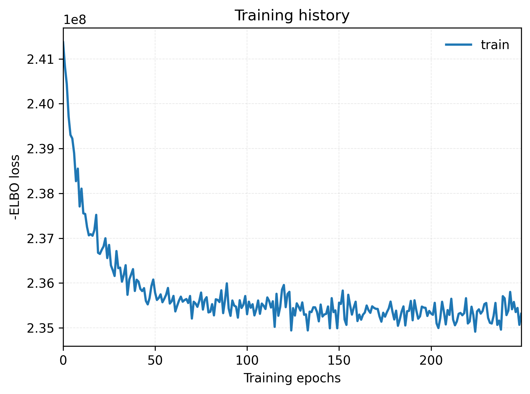
The ELBO curve displays the model training progress. The x-axis represents the number of training iterations and the y-axis represents the objective function value. This can be used to assess whether the reference model or spatial model has reached a relatively stable convergence state.

3. Dot plot linking abundances to unsupervised regions

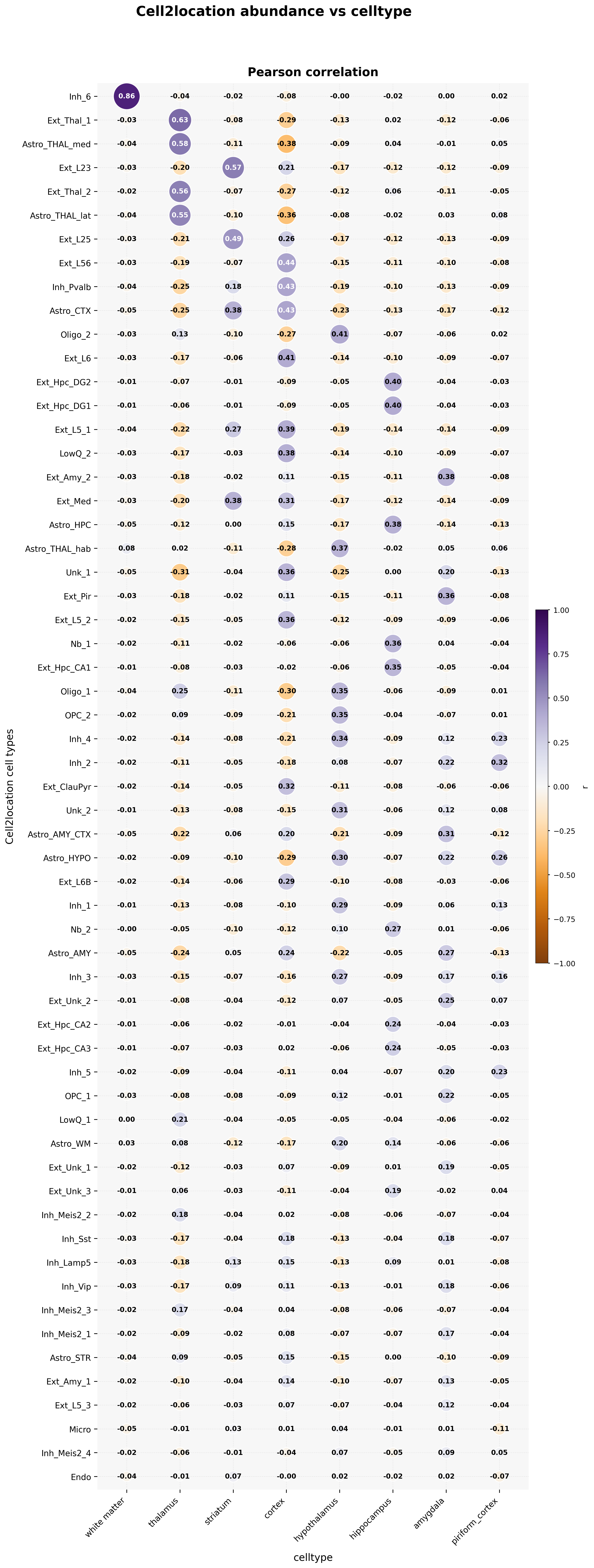
This figure summarizes the distribution characteristics of different cell types across different tissue regions. Different panels correspond to different cell types and can be used to identify spatial enrichment, continuous variation trends, and region-specific patterns.

4. Stacked bar plot of cell composition (`cluster_abundance_stacked_bar.png`)

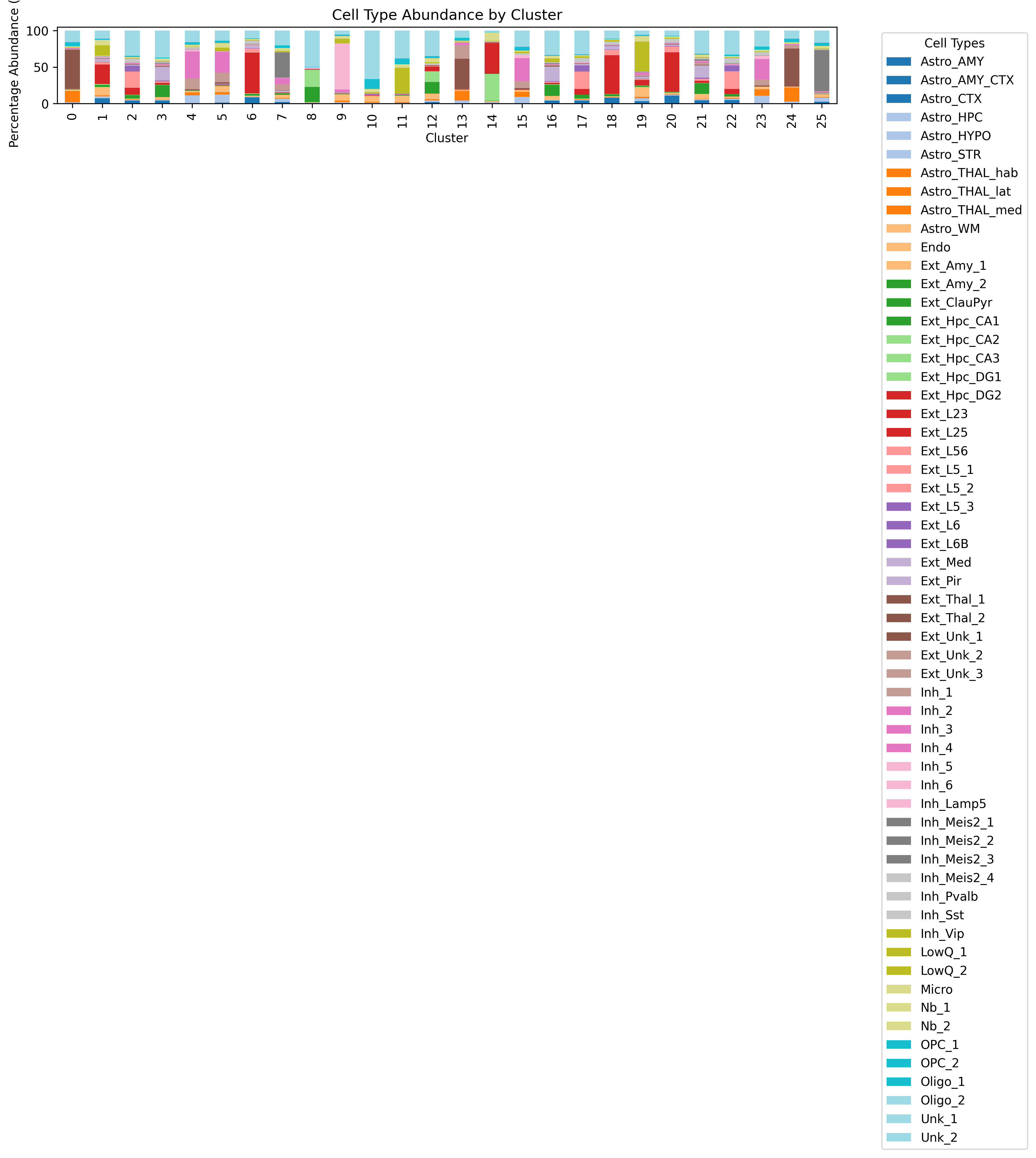
This stacked bar plot displays the relative abundance of each cell type across different clustering regions or samples and is suitable for comparing compositional differences between regions.

5. NMF-based decomposition analysis

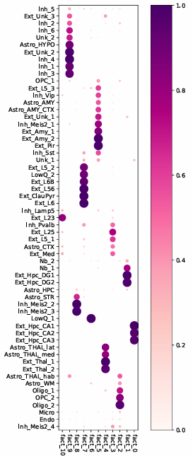
This result shows the latent composition patterns derived from further decomposition of the abundance matrix, which can assist in identifying representative cell co-localization structures and regional composition features.

6. Spatial visualization of decomposition factors

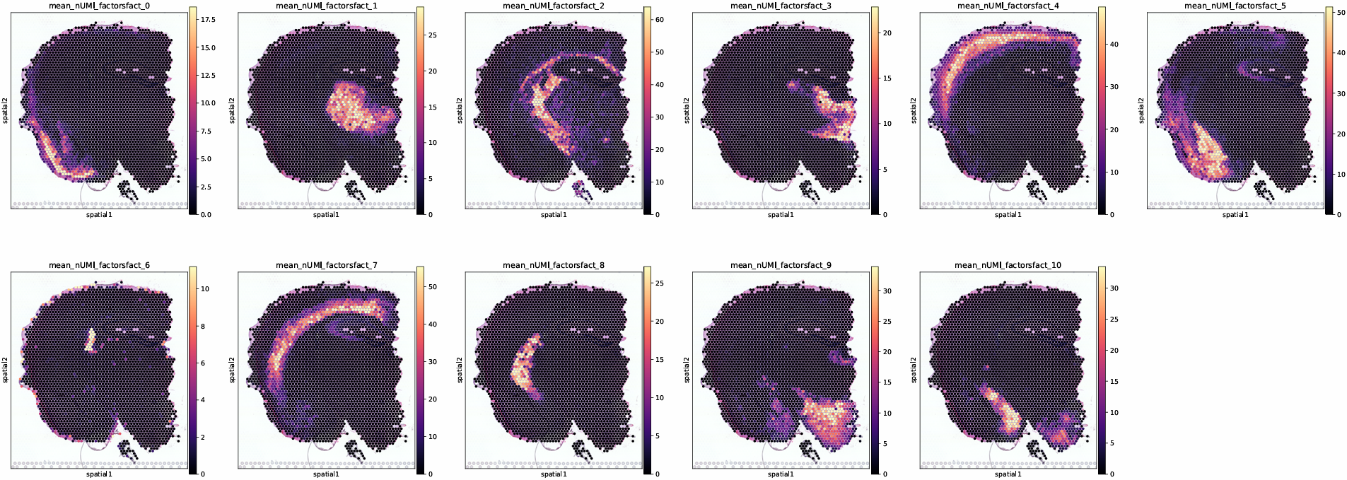
This figure maps the decomposed latent factors back onto spatial coordinates, helping to observe the spatial distribution of different composition patterns and their locally enriched regions.

7. Spatial map of dominant cell abundance

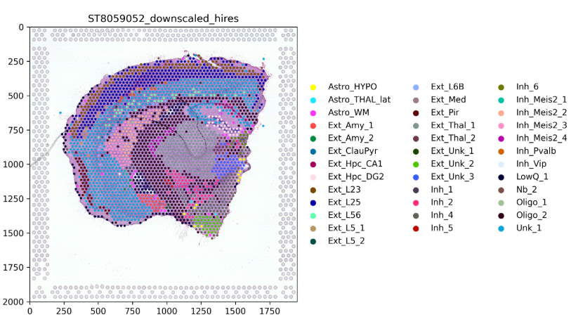
For low-resolution spatial data, cell2location returns cell abundance weights rather than discrete hard labels. This plot shows only the cell type with the highest abundance in each spot, serving as a rough overview of the overall spatial composition.

Algorithm-Based Annotation (cell2Location)

step 1: sample.txt configuration file