Clustering

Based on the preprocessed object, clustering builds the neighbor graph, generates low-dimensional visualizations, and performs unsupervised clustering. This is a central step for annotation and downstream biological interpretation. Because clustering quality directly affects annotation quality, we recommend testing the suggested number of PCs together with nearby values, such as the recommended value and recommended ± 5, and choosing the final setting based on boundary clarity, spatial continuity, and marker consistency.

Workflow overview

1. Read the filtered object generated in preprocess and construct the neighbor graph.

2. Represent the structure of the sample or integrated object in a low-dimensional embedding such as UMAP or tSNE.

3. Run clustering with the selected algorithm and write the labels back to the object.

4. Export visualization results and cluster labels for use in annotation_help.

Note

In this tutorial, we continue from the object generated in the previous preprocess step. If your data are not from the Visium HD platform, or if you are analyzing integrated multi-sample data, read through the following steps and replace the key parameters according to the command-line usage patterns introduced in previous tutorials.

Step 1: Configure sample.txt

You can directly reuse the same sample.txt configuration file from the integrate step; no modifications are needed.

sample_id input_path
sample_id data/sample_id

Step 2: Parameter Selection and Configuration

This step includes several important parameters. Please adjust them according to your needs. Below are some key parameters and their functions:

Parameter	Example	Description
--cluster_algorithm	leiden	Clustering algorithm; supported values include leiden, louvain, and Kmeans
--resolution	0.8	Community detection granularity for leiden or louvain, controlling clustering resolution
--n_clusters	15	Number of clusters used only for Kmeans
--pcs	25	Number of PCA dimensions used for clustering; adjust according to dataset size and computational resources, or use the value suggested in preprocess
--tsene	False	Whether to generate an additional tSNE visualization

Configuration recommendations:

1. For all scenarios: We recommend tuning pcs based on the pca_variance_ratio plot from the preprocess step and the recommended number of PCs printed in the terminal output. Our suggested default is 20, for reference only. Similarly, choose the clustering resolution according to your research goals; we recommend 0.8 as a balanced default that avoids both overfitting and underfitting.

2. The clustering module performs clustering and dimensionality reduction. To accommodate different analytical requirements, we provide multiple clustering algorithms including leiden, louvain, and Kmeans. Dimensionality reduction methods include UMAP and tSNE. You can select the clustering algorithm via --cluster_algorithm (default: leiden), and toggle tSNE visualization via --tsene (default: tsene False, meaning only UMAP is generated).

3. If you enabled sketch-based sampling in the preceding preprocess step, we recommend continuing with --sketch True in the clustering step to maintain a consistent downsampling strategy and project the clustering labels onto all spots/cells.

Parameter configuration methods:

1.The parameters listed above are commonly used settings that can be passed directly on the command line. If you are comfortable tuning spatial transcriptomics workflows, you can append them to the command as needed, for example --resolution 0.8.

2. Optional parameters through a configuration file. As introduced in the Usage tutorial, you can customize all parameters by editing a YAML configuration file before running the module. Use the command below to generate the YAML file for this step, then modify it as needed.

spatialsnake produce-file --option=clustering

After editing the configuration file, provide it on the command line with --configfile.

Step 3: Run the Command

Based on the command-line introductions in previous tutorials, you should now be familiar with the logic for setting key parameters in Spatialsnake. Here we only demonstrate running the clustering command. If you are working with multi-sample integration data or another platform, simply modify the relevant parameters accordingly. Remember to replace the example values with your chosen parameter settings or append them to the end of the command. For the example dataset, we use --resolution 0.8 --pcs 20 for single_analysis or visium_HD. This filters out spots or cells with fewer than 100 UMIs, fewer than 100 detected genes, or more than 30% mitochondrial signal.

spatialsnake single_analysis sample.txt visium_HD --option=clustering --resolution=0.8 --pcs=20

Run with a YAML file. Remember to save the edited YAML file before execution. No additional command-line arguments are required; if you do provide them, they will override the YAML values.

spatialsnake single_analysis sample.txt visium_HD --option=clustering --configfile=clustering.yaml

Demo for Clustering with visium_HD

We use the Colon_Cancer_P2_008um data ingested in the previous step for this clustering demonstration. The same sample.txt can be reused from the earlier analysis steps to maintain a consistent core analysis on the same sample.

sample_id input_path bin
Colon_Cancer_P2 data/Colon_Cancer_P2 8

We use the standard parameter set --resolution 0.8 --pcs 20 for clustering to identify cell types in the sample.

spatialsnake single_analysis sample.txt visium_HD --option=clustering --resolution=0.8 --pcs=20

If you prefer YAML-based configuration for more detailed parameter control:

# Generate and edit the YAML file
spatialsnake produce-file --option=clustering

spatialsnake single_analysis sample.txt visium_HD --option=clustering --configfile=clustering.yaml

Result file structure

This example shows single-sample clustering for visium_HD. After the run completes, first confirm that the clustered object can be loaded correctly, then judge whether the clustering is reasonable by combining the UMAP or tSNE view with the sample-by-cluster distribution plot.

results/
└── Colon_Cancer_P2_008um/
    └── clustering/
        ├── Colon_Cancer_P2.zarr/
        ├── Colon_Cancer_P2UMAP.png
        └── Colon_Cancer_P2Cell_Distribution_Across_Clusters.png

The output object {sample}.zarr (or concatenated_sdata in a multi-sample setting) contains the cluster labels in obs['clusters'] and serves as the direct input for annotation_help. If tsene=False, the tSNE plot is not generated.

Input and output structure

Analysis mode	Input	Output
single_analysis (standard zarr mode)	sample.txt should contain at least sample_id input_path; the input object is results/{sample}/preprocess/filter_{sample}.zarr	results/{sample}/clustering/{sample}.zarr
single_analysis (visium_HD)	sample.txt should contain at least sample_id input_path bin; the input object is results/{sample}_{bin}um/preprocess/filter_{sample}.zarr	results/{sample}_{bin}um/clustering/{sample}.zarr
compare_analysis	sample.txt should contain at least sample_id input_path group; for visium_HD, an additional bin column is required. The input object is results/merge_data/preprocess/filter_concatenated_sdata	results/merge_data/clustering/concatenated_sdata

How to inspect the clustering results

The UMAP plot is usually the first figure to inspect. Start by checking cluster boundaries, then evaluate whether the internal structure of each cluster is continuous and whether the global layout looks biologically plausible. A good clustering result typically shows clear boundaries, coherent within-cluster structure, and a natural overall organization.

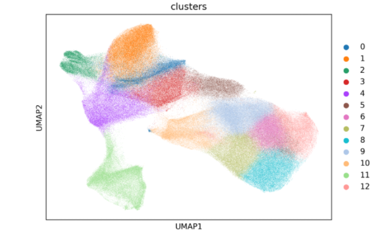
Key outputs

• Main object: results/{sample}_{bin}um/clustering/{sample}.zarr This object now contains obs['clusters'] and is the direct input for annotation_help.

• Visualization files: {sample}UMAP.png, {sample}Cell_Distribution_Across_Clusters.png, and {sample}tsene.png (optional) These plots are used to judge whether the clustering structure is clear and whether sample-specific bias is present.

Other outputs

1. {sample}Cell_Distribution_Across_Clusters.png (sample-by-cluster distribution)

   • This plot shows whether each cluster is distributed evenly across samples.

   • If a cluster appears almost exclusively in one sample, determine whether this reflects biology or technical bias.

   • In multi-sample analyses, interpret this figure together with the preprocessing results.

2. {sample}tsene.png (tSNE embedding)

   • This plot serves as a secondary check on the conclusions suggested by the UMAP plot.

   • If the overall pattern agrees with UMAP, confidence in clustering stability is usually higher.

   • If the two views differ strongly, revisit the clustering parameters and adjust them gradually.

Next, continue to Annotation Support.