Module 4: Spatial Domain Modeling (cellcharter)

cellcharter jointly leverages gene expression information and local spatial neighborhood structure to model spatial domains in tissue, thereby identifying spatial partitions that are more consistent with tissue organization. In addition to spatial domain identification, the pipeline also incorporates CellCharter’s enrichment analysis to compare cell-type enrichment patterns within a single sample or across multiple samples. In this tutorial, we use an already annotated example dataset to illustrate the spatial domain modeling workflow.

This module supports GPU acceleration. If running in a CPU-only environment, the overall runtime will typically increase substantially.

For the complete parameter configuration reference, see advance_analysis.yaml Reference.

1. Read and preprocess the input object.

2. Construct a feature representation that incorporates spatial neighborhood information.

3. Evaluate stability across a range of candidate cluster numbers and select the most appropriate number of spatial domains.

4. Output single-sample or multi-sample comparison results according to the run branch.

More specifically, the pipeline reads a .zarr or .h5ad object, normalizes the expression matrix, and builds a counts layer. It then constructs a spatial neighborhood graph and integrates the cell’s or spot’s own expression with the neighborhood context into X_cellcharter features. Clustering stability is evaluated over the range (2, max_cluster) to determine the final number of spatial domains. Finally, depending on the single-sample or multi-sample analysis mode, it outputs spatial partition plots, neighborhood enrichment plots, and comparative results.

step 1: sample.txt configuration file

The recommended sample.txt format is as follows; replace {sample_id} with your own sample ID:

sample_id   input_path
{sample_id} results/{sample_id}/annotation/{sample_id}.zarr

Input requirements:

1. The input object must contain spatial coordinate information, which may be stored in obsm['spatial'] or other equivalent convertible fields.

2. It is recommended to use an object that already contains celltype annotations to ensure that enrichment results have clear biological interpretability.

3. For multi-sample comparison analysis, it is recommended to use an integrated object and retain both the sample column and the experimental condition or grouping column, e.g., sample_col=region and condition_col=condition (if your data were integrated through Spatialsnake, the default parameters can be used as is).

Step 2: Parameter Selection and Configuration

In the CellCharter module, the following parameters are usually the most important to understand first:

Parameter	Example	Description
runpipe	cellcharter	Specifies the current advanced analysis branch as CellCharter
max_cluster	10	Upper limit for the number of candidate spatial domains; used for automatic evaluation of the optimal number of clusters
significance	0.05	Significance threshold for enrichment results
condition_col	condition	Column name used to define condition groups in multi-sample comparison mode
sample_col	region	Column name used to identify sample origin in multi-sample comparison mode
celltype_col	celltype	Column name of the cell-type annotation in the input object, used for enrichment analysis
cellcharter_col	spatial_cluster	Column name used when writing CellCharter spatial domain labels back into the object
image_type	hires	Image layer used for spatial overlay display
shape_type	cell_boundaries	Layer used for spatial boundary visualization

Configuration recommendations:

1. max_cluster directly affects the range over which the number of spatial domains is automatically selected. If the tissue structure is more complex, it can be increased moderately; if the sample size is small, it should not be set too high.

2. If you are interested in spatial organization differences between conditions, condition_col and sample_col must be accurately set; otherwise robust cross-condition enrichment comparison results cannot be generated.

3. celltype_col and cellcharter_col respectively determine the read/write logic for input annotations and output spatial domain labels, and are the most critical column-name parameters for interpreting results.

A typical configuration example:

image_type: "hires"
shape_type: "cell_boundaries"
significance: 0.05
max_cluster: 10
condition_col: "condition"
sample_col: "region"
celltype_col: "celltype"
cellcharter_col: "spatial_cluster"

Step 3: Run the Command

Once input preparation and parameter confirmation are complete, run:

spatialsnake single_analysis sample.txt visium --option=advance_analysis --runpipe=cellcharter

Using the annotated example spatial object, the following demonstrates the standard CellCharter workflow.

1. Prepare the input object

We use Colon_Cancer_P2_008um from the core analysis annotation step as the example dataset. Ensure that the preceding core analysis and annotation steps have already been completed.

sample.txt:

sample_id   input_path
Colon_Cancer_P2_008um results/Colon_Cancer_P2_008um/annotation/Colon_Cancer_P2.zarr

2. Set the key parameters

For this demonstration, the default parameters are sufficient. For other samples, adjust the parameters as appropriate.

3. Run CellCharter

spatialsnake single_analysis sample.txt visium --option=advance_analysis --runpipe=cellcharter

Spatialsnake uses GPU acceleration automatically when a GPU is available. If no GPU is detected, it falls back to CPU computation. Ensure that sufficient GPU memory is available when running the accelerated version.

Result file structure

Single-sample output (default mode):

results/
└── Colon_Cancer_P2_008um/
      └── cellcharter/
            ├── Colon_Cancer_P2_008um_cellcharter.zarr/
            ├── Colon_Cancer_P2_008um_celchar.png
            ├── Colon_Cancer_P2_008um_enrichment.png
            ├── Colon_Cancer_P2_008um_nhood_enrichment.png
            ├── Colon_Cancer_P2_008um_Clusters.png
            └── Colon_Cancer_P2_008um_cell_clusters.csv

Here, {sample}_diff_enrichment.png is generated only when all of the following conditions are met simultaneously:

1. The pipeline is running in the multi-sample comparison branch (channel=compare_analysis).

2. condition_col in the input object contains at least two condition groups.

3. sample_col is present in the input object to support sample-level neighborhood comparison.

1. Clustering stability plot

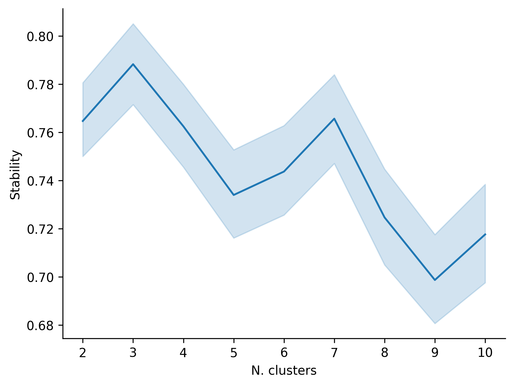
This figure displays the stability of different candidate cluster numbers across repeated runs and is used to judge whether the final selected number of spatial domains is reliable.

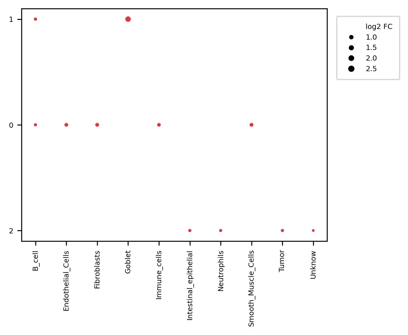
2. Neighborhood enrichment plot

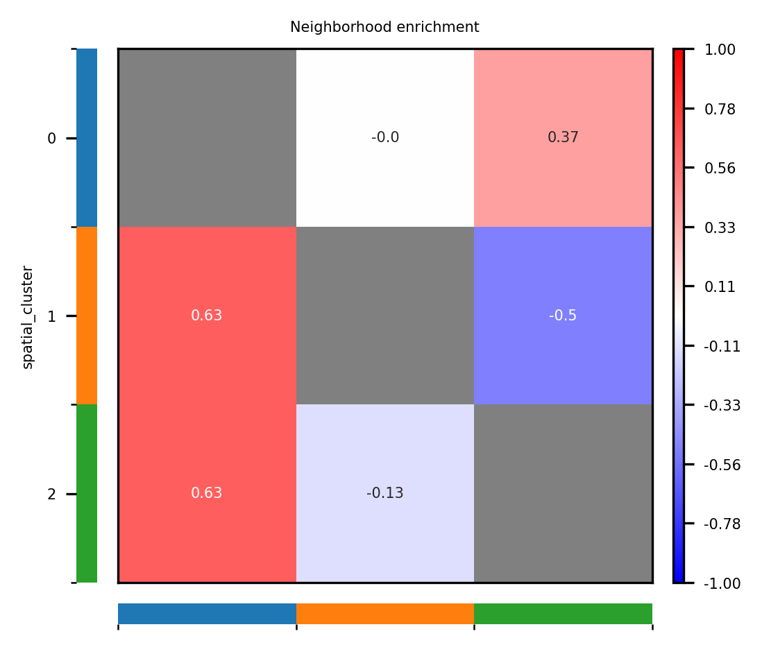
This figure displays adjacency enrichment or exclusion relationships among different spatial domains and helps identify co-localization patterns or mutually exclusive structures within the tissue microenvironment.

3. Condition-specific enrichment plot

In multi-sample mode, CellCharter generates enrichment plots separately for each condition_col group, making it possible to observe the spatial tissue organization within each condition.

4. Differential neighborhood enrichment plot

This figure compares neighborhood enrichment differences between conditions and highlights domain-domain relationships that change significantly. It is one of the most important results in comparative spatial analysis.

5. Spatial overlay plot

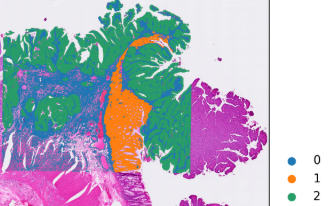
This figure overlays the spatial domain labels on the tissue image and can be used to assess whether the inferred spatial partitions are consistent with the tissue morphology, and to further assign biological interpretation to each domain.