Annotation Support

Based on the clustering results, annotation_help performs marker gene statistics, enrichment analysis, and spatial cluster visualization to provide interpretable biological evidence for the downstream annotation step. In a single-sample setting, this stage helps identify candidate cell types for each cluster. In an integrated multi-sample setting, it also helps assess whether marker and pathway results are influenced by sample composition.

This stage combines both Python and R tools. If the R environment has not yet been configured, use conda to install relevant R packages:

Workflow overview

Read the output object from clustering together with the clusters labels.
Compute differential marker genes by cluster and export both a combined table and per-cluster tables.
Generate marker dotplots, sample-by-cluster proportion plots, and spatial overlay figures.
Run KEGG enrichment analysis based on the marker genes and export pathway results.
Write all annotation support outputs into the clustering directory so that they can be used directly by annotation.

Step 1: Configure `sample.txt`

You can directly reuse the same sample.txt configuration file from the integrate step; no modifications are needed.

sample_id input_path
sample_id data/sample_id

Step 2: Parameter Selection and Configuration

This step includes several important parameters. Please adjust them according to your needs. Below are some key parameters and their functions:

Parameter	Example	Description
`--markers_algorithm`	`wilcoxon`	Marker statistics method; `wilcoxon` is commonly used, but `t-test` and others can also be selected when appropriate
`--species`	`human`	Species background used for enrichment analysis, typically `human` or `mouse`

These parameters are passed directly to annotation_help and the enrichment workflow. If you want to switch strategies quickly, append them to the command, for example --markers_algorithm=t-test --species=mouse.

Configuration recommendations:

This step performs differential expression analysis between clusters and gene set enrichment analysis to characterize the expression signatures of each cluster and assist in the interpretation of cluster identity and cell-type assignment.
The default parameters are generally sufficient. If you wish to customize the configuration, consider the markers_algorithm and species parameters to specify the differential analysis method and the species background. Both human and mouse are supported.
If your study involves other species or requires additional parameters for more detailed differential gene analysis, please contact us.

Parameter configuration methods:

1.The parameters listed above are commonly used settings that can be passed directly on the command line. If you are comfortable tuning spatial transcriptomics workflows, you can append them to the command as needed, for example --markers_algorithm=t-test --species=mouse.

2. Optional parameters through a configuration file. See annotation_help.yaml Reference for the full parameter reference. Generate a YAML template with: The YAML file contains inline comments describing each parameter. You can adjust the settings according to your analysis needs, or consult the corresponding configuration reference page for detailed explanations. After editing the configuration file, provide it on the command line with --configfile.

spatialsnake produce-file --option=annotation_help

Step 3: Run the Command

Based on the command-line introductions in previous tutorials, you should now be familiar with the logic for setting key parameters in Spatialsnake. Here we only demonstrate running the annotation_help command. If you are working with multi-sample integration data or another platform, simply modify the relevant parameters accordingly. Remember to replace the example values with your chosen parameter settings or append them to the end of the command. For the example dataset, we use --markers_algorithm=t-test --species=human for single_analysis or visium_HD.

spatialsnake single_analysis sample.txt visium_HD --option=annotation_help --markers_algorithm=t-test --species=mouse

Run with a YAML file. Remember to save the edited YAML file before execution. No additional command-line arguments are required; if you do provide them, they will override the YAML values.

spatialsnake single_analysis sample.txt visium_HD --option=annotation_help --configfile=annotation_help.yaml

Demo for annotation_help with visium_HD

We use the Colon_Cancer_P2_008um data from the previous step for this annotation_help demonstration. The same sample.txt can be reused from the earlier analysis steps to maintain a consistent core analysis on the same sample.

sample_id input_path bin
Colon_Cancer_P2 data/Colon_Cancer_P2 8

spatialsnake single_analysis sample.txt visium_HD --option=annotation_help

If you prefer YAML-based configuration for more detailed parameter control:

# Generate and edit the YAML file
spatialsnake produce-file --option=annotation_help

spatialsnake single_analysis sample.txt visium_HD --option=annotation_help --configfile=annotation_help.yaml

Result file structure

This example shows single-sample annotation support for visium_HD. Before moving to manual annotation, first confirm that marker_genes_pval.csv and kegg_data.csv have been generated. The workflow creates one subdirectory for each cluster, containing its differential marker table, KEGG enrichment results, spatial visualization outputs, and related files, making it easier to interpret the characteristic features of each candidate cell type.

results/
└── Colon_Cancer_P2_008um/
    └── clustering/
        ├── marker_genes_pval.csv
        ├── kegg_data.csv
        ├── Colon_Cancer_P2rank_genes_groups_dotplot.png
        ├── Clusters_proportion.png
        ├── Colon_Cancer_P2_hires_image_cluster.png
        ├── [cluster_id]/
        │   └── cluster_[cluster_id].csv
        └── clusters.csv

Note

The main core analysis workflow is now complete. The annotation support results are stored in the clustering directory. Next, continue to Annotation Modules for manual annotation or algorithm-based annotation.

Key parameter recommendations

Parameter category	Recommendation for single-sample analysis	Recommendation for multi-sample or cross-condition analysis
`--markers_algorithm`	`wilcoxon` is usually preferred because it is stable and easy to interpret	Use the same method across all samples to reduce comparison bias
`--species`	Match the species of the dataset, usually `human` or `mouse`	Keep this consistent across all samples or enrichment results will not be directly comparable
`image_type` / `shape_type` (YAML)	Usually keep the default settings and complete the global analysis first	For integrated objects, use a consistent layer type to avoid interpretation shifts caused by different visualization baselines
`image_slice` (YAML parameter)	Usually keep it disabled to inspect the full structure first	Enable it only when focusing on a target region, and record the crop coordinates for reproducibility

Input and output structure

After clustering is complete, you can usually reuse the same sample.txt file for annotation_help.

Analysis mode	Input	Output
single_analysis (standard `zarr` mode)	`sample.txt` should contain at least `sample_id input_path`; the input object is `results/{sample}/clustering/{sample}.zarr`	`results/{sample}/clustering/marker_genes_pval.csv` and `results/{sample}/clustering/kegg_data.csv`
single_analysis (`visium_HD`)	`sample.txt` should contain at least `sample_id input_path bin`; the input object is `results/{sample}_{bin}um/clustering/{sample}.zarr`	`results/{sample}_{bin}um/clustering/marker_genes_pval.csv` and `results/{sample}_{bin}um/clustering/kegg_data.csv`
compare_analysis	`sample.txt` should contain at least `sample_id input_path group`; for `visium_HD`, an additional `bin` column is required. The input object is `results/merge_data/clustering/concatenated_sdata`	`results/merge_data/clustering/marker_genes_pval.csv` and `results/merge_data/clustering/kegg_data.csv`

How to inspect the results

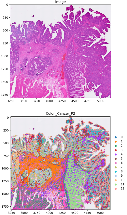
This step produces a spatial cluster map showing the tissue distribution of each cluster. The figure panels typically include the original H&E-stained image together with the mapped cluster assignments, allowing you to interpret the spatial organization of the clusters in histological context.

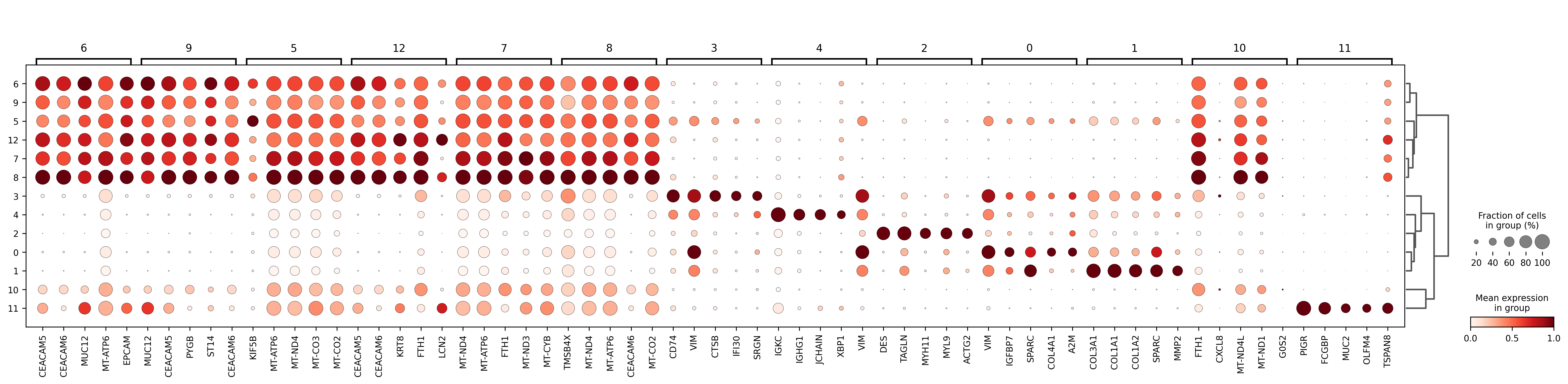
The marker dotplot summarizes the strength and specificity of representative genes across clusters. You can combine it with the exported CSV tables to determine the defining markers for each cluster before annotation.

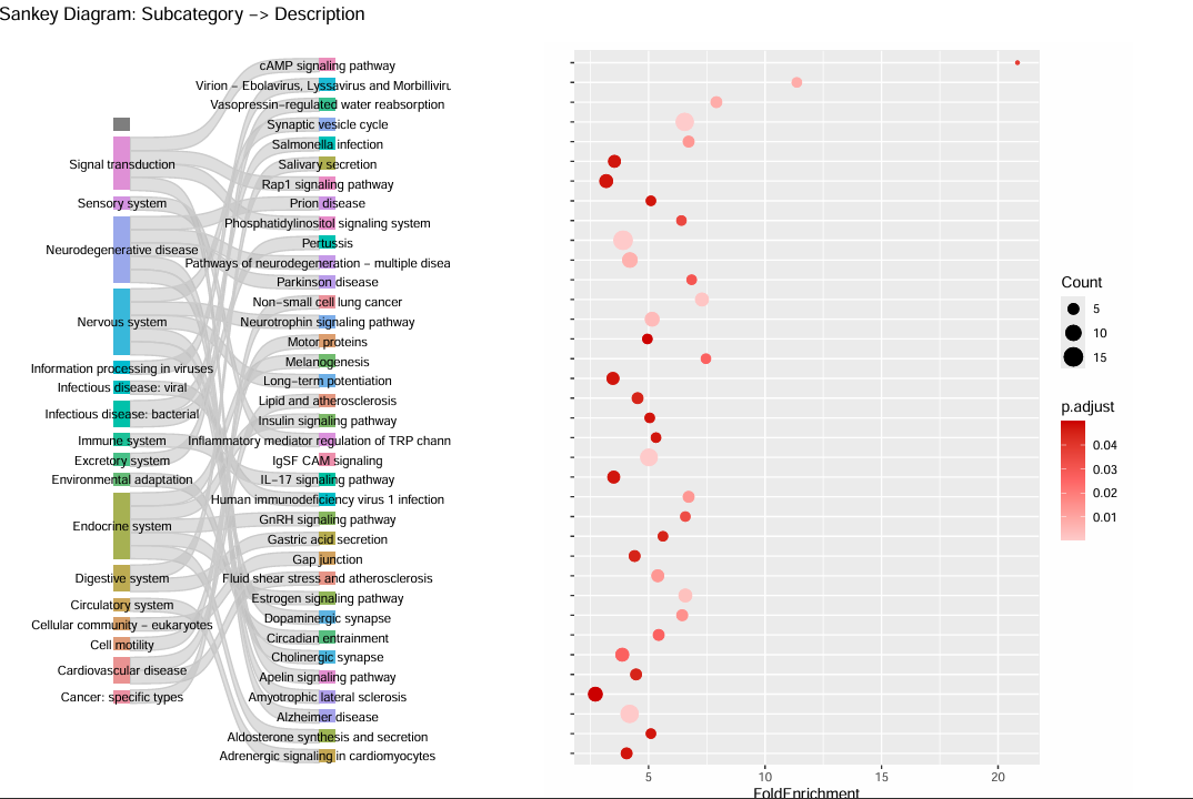
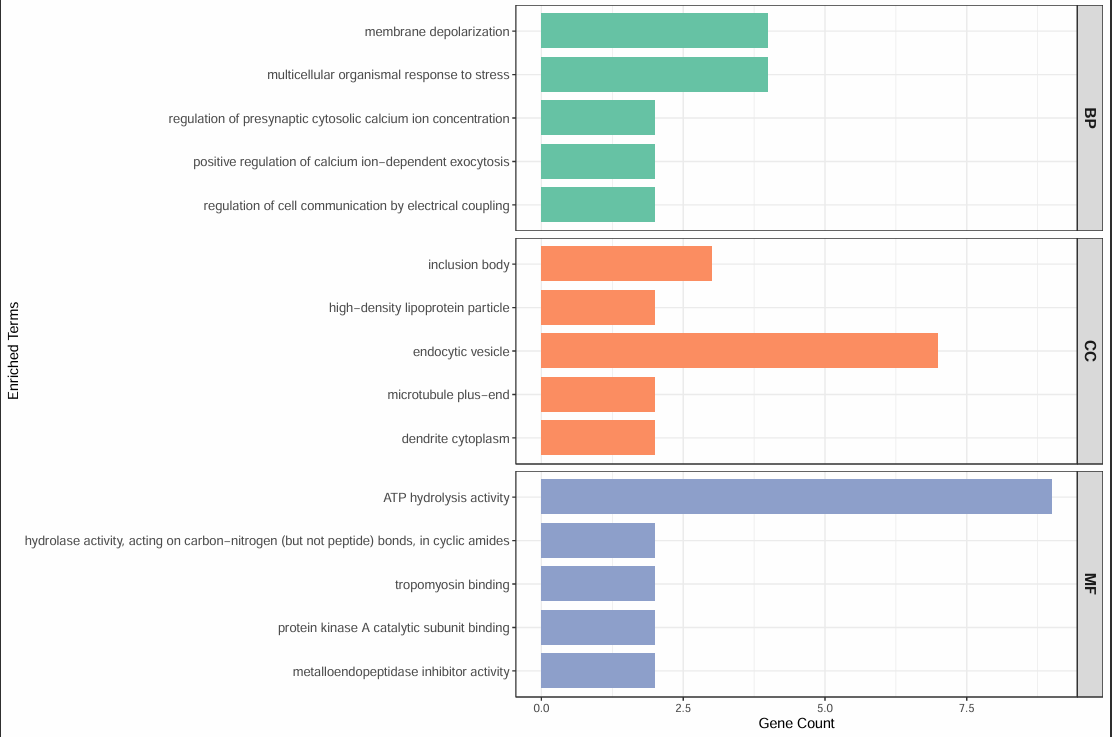
Each cluster-specific directory also contains differential marker tables and GO/KEGG enrichment results, helping you interpret the most enriched pathways for that cluster.

annotation help remaining plots placeholder

Other outputs

marker_genes_pval.csv (combined marker table)
- This is the main evidence table for annotation and summarizes the most representative genes for each cluster.
- Prioritize gene combinations that appear consistently and agree with known cell-type characteristics.
- In most cases, this table forms the primary basis for assigning cell-type names.
<cluster_id>/cluster_<cluster_id>.csv (per-cluster marker table)
- This file isolates each cluster into its own table for detailed inspection.
- Cluster-specific review makes it easier to detect mixed signatures.
- If one cluster contains multiple incompatible signals, revisit the upstream clustering settings and consider whether the clustering is too coarse.
kegg_data.csv (pathway enrichment)
- This table provides additional evidence about the biological processes associated with each cluster.
- Pathway results should be interpreted together with marker genes rather than used alone for annotation.
- If pathway and marker evidence clearly conflict, re-evaluate clustering quality before assigning labels.
{sample}rank_genes_groups_dotplot.png (global expression pattern overview)
- This plot helps you quickly see which genes are strongest in which clusters.
- If some genes are clearly enriched in only one target cluster, annotation confidence is usually higher.
- If several clusters share similar expression patterns, finer subclustering may still be useful.
Clusters_proportion.png and [image]_Clusters.png (composition and spatial distribution)
- The cluster proportion plot shows compositional differences across samples or regions.
- The spatial overlay figure helps verify whether cluster locations are coherent and consistent with tissue structure.
- When composition patterns and spatial localization support the same interpretation, the data are usually ready for manual annotation.

Continue to Annotation Modules.