Module 6: Cell Communication Network Analysis (cellchat)
cellchat is a downstream module for cell-cell communication analysis. It infers signaling relationships from ligand-receptor pairs and summarizes the strength of communication between cell populations.
For spatial transcriptomics data, the workflow also accounts for physical distance between spots or cells across different platforms, allowing the inferred communication probabilities to better reflect tissue architecture.
What This Module Does
Load the annotated expression object The input object must already contain cell-type labels or another biologically meaningful grouping variable.
Define communication groups CellChat uses the selected annotation column to determine which cell populations will act as candidate senders and receivers.
Match ligand-receptor information The workflow selects the species-specific communication database and searches for signaling relationships supported by the observed expression data.
Incorporate spatial structure when applicable For spatial data, the workflow uses spot or cell coordinates together with platform-appropriate spatial scaling information.
Estimate communication probability Interaction strength is inferred at the ligand-receptor level and then summarized to signaling pathways and cell-group networks.
Generate interpretable outputs The module produces network plots, pathway summaries, heatmaps, and ligand-receptor tables for biological interpretation.
Note
This module generates the core figures and CSV tables required to summarize ligand-receptor communication in the current dataset.
For more detailed visualization, or to compare communication strength across experimental conditions, continue to Module 8: Comparative Communication Analysis (compare_stage + cellchat).
That downstream comparison step uses the cellchat.rds object produced here as its input.
For datasets with different experimental conditions, run this module separately for each condition first. Integrated CellChat analysis in this step is intended only for biological replicates from the same condition.
How To Prepare and Run This Module
Step 1. Confirm the analysis scenario
Before preparing files, first decide which of the following scenarios matches your study design:
Single-cell data Use this setting when the data contain no spatial coordinates. In this case, the module focuses entirely on expression-defined communication and does not require spatial scaling information.
Single spatial sample Use this setting when the goal is to characterize communication within a single tissue section. Spatialsnake automatically reads the spatial coordinates from the sample object and uses them to constrain communication distance.
Multiple spatial samples from the same condition Use this setting only for biological replicates from the same condition. The resulting network represents the integrated communication pattern of that condition rather than a between-condition comparison.
The spatial transcriptomics platform used in the analysis
Important
Multiple spatial samples should be integrated in this module only when they belong to the same biological condition. If the goal is to compare two or more different conditions, first run CellChat separately for each condition and then perform downstream comparative analysis.
Step 2. Prepare the input object
The input object should already be annotated and ready for downstream communication analysis. In practical terms, this means:
Ensure that the spatial transcriptomics object has completed the annotation step and contains an annotation column.
The default input format is standard
h5ad, and the default annotation column iscelltype. If your data are stored in another format, convert them in advance using the format-conversion tool.Confirm the platform used for your spatial data and ensure that standard coordinate information is available, as
st_cellchatrequires spatial coordinates for analysis.
Step 3. Write sample.txt according to platform
The sample.txt differs across platforms
We synthesized recommendations from the CellChat authors together with guidance from GitHub community discussions to optimize the workflow for spatial transcriptomics analysis. Because spot or cell spacing differs across platforms, different parameter settings are required for accurate communication modeling. Users therefore need to provide the appropriate platform field or bin size so that the workflow can select the most suitable spatial settings automatically. This design also reduces manual tuning and allows users to focus on biological interpretation.
Visium-family platforms The coordinates are linked to image resolution and spot geometry. Therefore, a scale-factor description is needed to translate coordinate distances into spot-scale distances.
Stereo-seq The key spatial unit is often a bin or a cell-bin definition. The workflow therefore expects a bin-related specification rather than an image-derived scale-factor file.
MERFISH, MERSCOPE, and Xenium These platforms usually provide coordinates at higher spatial resolution, often approaching single-cell resolution. The workflow can therefore rely more directly on platform defaults for spatial scaling, and an additional third-column specification is typically unnecessary.
Visium-family platforms
Single spatial sample:
sample_id    input_path    scale_factor
SampleA    /path/to/SampleA.h5ad    /path/to/SampleA_scalefactors_json.json
Multiple spatial replicates from the same condition:
sample_id    input_path    scale_factor
Rep1    /path/to/concatenated_sdata.zarr    /path/to/Rep1_scalefactors_json.json
Rep2    /path/to/concatenated_sdata.zarr    /path/to/Rep2_scalefactors_json.json
Rep3    /path/to/concatenated_sdata.zarr    /path/to/Rep3_scalefactors_json.json
Explanation: The third column should contain the scale-factor description associated with each sample. For Visium-family data, communication distance should be calibrated relative to the physical spot geometry rather than raw image coordinates alone.
Stereo-seq
Single bin-based sample:
sample_id    input_path    bin_or_cellbin
StereoA    /path/to/StereoA.h5ad    50
Single cell-bin sample:
sample_id    input_path    bin_or_cellbin
StereoCellBin    /path/to/StereoCellBin.h5ad    cellbin
Multiple Stereo-seq replicates from the same condition:
sample_id    input_path    bin_or_cellbin
Rep1    /path/to/concatenated_sdata.zarr    50
Rep2    /path/to/concatenated_sdata.zarr    50
Rep3    /path/to/concatenated_sdata.zarr    50
Explanation:
For Stereo-seq, the third column is not an image scale-factor file. Instead, it records the spatial aggregation unit, usually a bin size or cellbin. This directly determines how the workflow interprets the physical size of each observation and therefore affects spatial communication modeling.
MERFISH, MERSCOPE, and Xenium
Single spatial sample:
sample_id    input_path
XeniumA    /path/to/XeniumA.h5ad
Multiple spatial replicates from the same condition:
sample_id    input_path
Rep1    /path/to/concatenated_sdata.zarr
Rep2    /path/to/concatenated_sdata.zarr
Rep3    /path/to/concatenated_sdata.zarr
Explanation: These platforms usually provide higher-resolution coordinates, so the workflow can generally proceed without an additional third-column specification. In these cases, spatial scaling is handled using platform-level defaults.
Single-cell data
Single dataset:
sample_id    input_path
sc_sample    /path/to/sc_sample.rds
Explanation: Because there is no spatial geometry in standard single-cell data, no third column is needed for spatial calibration.
Platform-specific spatial parameters and auto-selection logic
In CellChat spatial analysis, spot.diameter represents the effective physical size of one observation unit.
This value cannot be shared across platforms because different technologies do not measure the tissue at the same spatial resolution.
Some platforms summarize transcripts in relatively large spots, whereas others work at bin-level or near single-cell resolution.
As a result, the same coordinate distance can correspond to very different biological distances across platforms.
According to the official CellChat spatial tutorial and the discussion in issue #6, spatial distances should be interpreted on a biologically meaningful scale.
Therefore, spot.diameter should be set either from an officially provided platform description or from a platform-specific calculation based on the true spatial unit.
How spot.diameter is selected for each platform
The table below summarizes which parameters are automatically adjusted according to the underlying platform technology.
Platform |
Selection type |
Basis |
Current workflow behavior |
|---|---|---|---|
|
Official recommendation |
Standard spot diameter defined by the platform |
Uses |
|
Calculated from dataset naming or user setting |
Effective bin size may differ by dataset |
First tries to infer the bin size from the input name; if not available, falls back to the configured |
|
Practical default with optional override |
Observation units are smaller than standard Visium spots |
Uses the Visium-family scale-factor branch but defaults to a smaller observation size unless the user provides a custom value |
|
Platform-specific calculation |
The true spatial unit depends on the bin definition |
Reads the third column as a positive bin size and converts it internally to the effective |
|
Platform-specific calculation |
The observation unit is a cell-bin rather than a classical spot |
Reads the third column as |
|
Practical default with optional override |
These platforms are already high resolution and closer to cell-level coordinates |
Uses a small default |
In short, spot.diameter should always match the real biological observation unit of the platform rather than the raw coordinate number itself.
Step 4. Configure key parameters
For the configuration reference, see advance_analysis.yaml Reference.
The following parameters are the most important for routine use:
Parameter |
Typical values |
Description |
|---|---|---|
|
|
Selects the CellChat branch |
|
|
Annotation column used to define communicating cell groups |
|
|
Selects the species-specific ligand-receptor database |
|
|
Indicates the analysis context used by the module |
|
|
Filters out very small cell groups that are unlikely to support robust communication inference |
|
A moderate or high integer depending on available CPU resources |
Controls parallel computation |
|
|
Switches between spatial mode and single-cell mode |
|
|
Controls robustness of the truncated-mean strategy used during probability estimation |
|
Platform- and tissue-dependent |
Sets the effective spatial communication range in spatial mode |
|
Platform-dependent |
Represents the effective observation diameter or cell-size proxy used for spatial scaling |
Copyable configuration examples
Single spatial sample:
celltype_col: "celltype"
species: "human"
is_single_cell: False # default is False
interaction_length: 200 # distance limit; choose according to platform-specific spatial scale
min_cells: 10
trim: 0.1
Single-cell mode:
# cellchat
celltype_col: "celltype"
assay: "Spatial"
species: "human"
min_cells: 10
workers: 32
is_single_cell: True
trim: 0.1
interaction_length: 250
Single-cell dataset:
First set cellchat_is_single_cell: True in the configuration file, then run:
Spatial dataset:
spatialsnake single_analysis sample.txt visium --option=advance_analysis --runpipe=cellchat
Result file structure
The module produces one communication-analysis result set for each run. The main output categories are:
Serialized CellChat object This object preserves the inferred communication model and can be reused in subsequent comparative analyses.
Network overview figures These summarize the number and strength of interactions among cell groups.
Pathway-level summary figures These show which signaling programs dominate the current dataset.
Heatmaps and signaling-role plots These help interpret sender, receiver, and pathway-centrality patterns.
Ligand-receptor and pathway summary tables These provide the tabular evidence required for downstream validation, filtering, and biological reporting.
How to interpret the results
1. Network overview plot
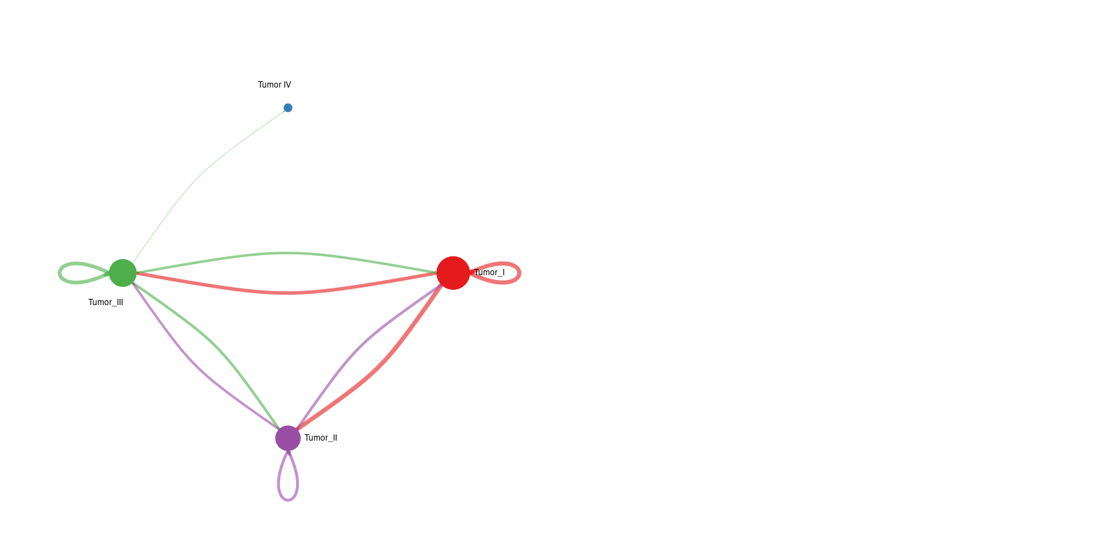
Interpretation: The left panel shows the number of interactions between cell groups, whereas the right panel shows interaction strength. Together, these figures provide a rapid overview of communication hubs and dominant sender-receiver relationships.
2. Information-flow bar plot

Interpretation: This plot compares information flow across signaling pathways and helps prioritize the most active or biologically relevant communication programs.
3. Communication heatmaps
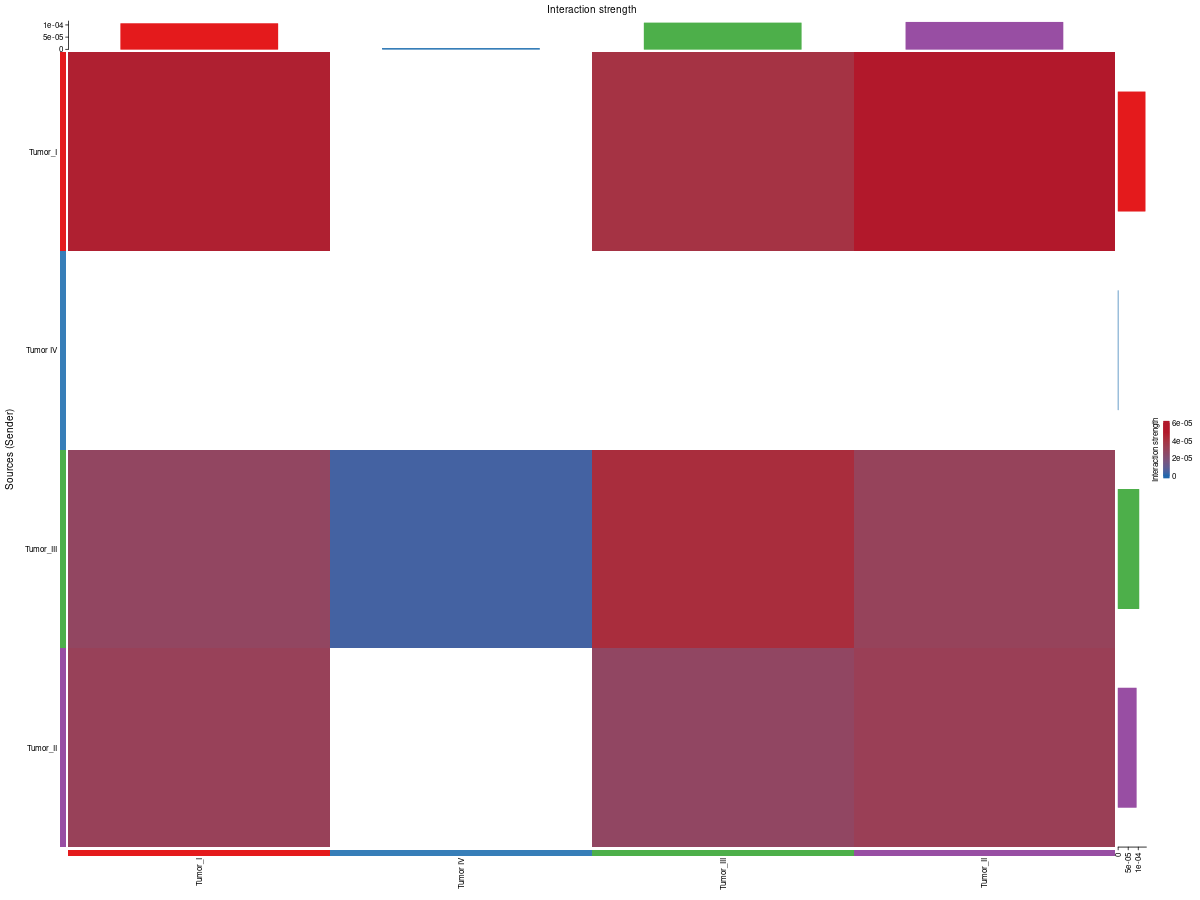
Interpretation:
count_heatmap summarizes the number of interactions between cell groups, whereas cellchat_heatmap summarizes interaction strength. Viewed together, they help distinguish communication programs that are widespread but weak from those that are sparse but strong.
4. Signaling-role plots
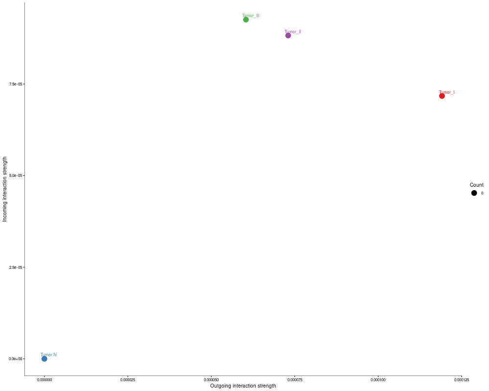
Interpretation: For one automatically selected signaling pathway, the workflow generates network, scatter, outgoing, and incoming role plots. These figures help identify which cell groups act as senders, receivers, or central intermediates within that pathway.
5. LR-level detail and summary statistics
Interpretation:
lr.csv contains ligand-receptor evidence at the individual interaction level, whereas lr_summary.csv provides aggregated interaction strength and significance for each LR pair. Together, these files form a primary basis for mechanistic interpretation and reproducible downstream analysis.